Normal moveout

A seismic trace represents a signal d(t) recorded at a constant location x. The normal moveout operator transforms a trace into a ``vertical propagation'' signal, $m(\tau) = d(t)$, by stretching t into $\tau$ Claerbout (1999). For conventional PP seismic processing the NMO transformation is generally described as a hyperbola. For PS waves the traveltime moveout does not approximate a hyperbola for large values of offset-to-depth ratio even for an Earth's model consisting on horizontal layers embedded in a constant P and S velocities.

One of the main characteristic of converted-wave data is their non-hyperbolic moveout in CMP gathers. However, for certain values of offset-to-depth ratio, it is possible to approximate the non-hyperbolic moveout in a CMP gather to a hyperbola Tessmer and Behle (1988).

Castle (1988) developed a non-hyperbolic moveout equation for converted-wave data. This equation consists on three coefficients instead of the two coefficients for the hyperbolic equation. Castle's 1988 non-hyperbolic moveout equation is a function of both the P-velocity and the S-velocity. Next, I present an expression for the non-hyperbolic moveout equation in terms of $\gamma$.

Equation is the third-order approximation for the total traveltime function of reflected PP or SS data presented by Taner and Koehler (1969):

 

t² = c₁ + c₂ x² + c₃ x⁴, (1)

where x represents surface-offset, the first coefficient c₁ = b₁², the second coefficient $c_2 = \frac{b_1}{b_2}$, and the third coefficient $c_3 = \frac{b_2^2 - b_1 b_3}{4b_2^4}$, where

$$b_m = \sum_{k=1}^n z_k \left ( v_{p_k}^{2m-3}+v_{s_k}^{2m-3} \right ).$$ (2)

The summation index k indicates the stratigraphic layers in the model, v_p is the vertical P-velocity, and v_s is the S-velocity.

For the second order approximation of the total traveltime function, Tessmer and Behle (1988) show that the first coefficient, c₁, is simplified as  

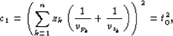$$c_1 = \left ( \sum_{k=1}^n z_k \left ( \frac{1}{v_{p_k}} + \frac{1}{v_{s_k}} \right ) \right )^2 = t_0^2,$$ (3)

and the second coefficient, c₂, reduces to  

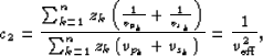$$c_2 = \frac{\sum_{k=1}^n z_k \left ( \frac{1}{v_{p_k}} + \fr... ...k \left (v_{p_k} + v_{s_k} \right )} = \frac{1}{v_{\rm eff}^2},$$ (4)

where $v_{\rm eff}^2=v_p \cdot v_s$. This simplification for the second coefficient (c₂) is valid only for constant values of $\gamma$.

The third coefficient, as presented by Castle (1988), is  

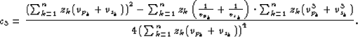$$c_3 = \frac{\left (\sum_{k=1}^n z_k (v_{p_k} + v_{s_k}) \rig... ...3)}{4 \left ( \sum_{k=1}^n z_k (v_{p_k} + v_{s_k}) \right )^4}.$$ (5)

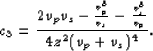
For one layer, equation  simplifies to

$$c_3 = \frac{z^2 \left [ (v_p+v_s)^2 - (\frac{1}{v_p} + \frac{1}{v_s})(v_p^3 + v_s^3) \right ]}{4 z^4 (v_p+v_s)^4},$$ (6)

which reduces to

 

$$c_3 = \frac{2 v_p v_s - \frac{v_p^3}{v_s} - \frac{v_s^3}{v_p}}{4z^2 (v_p+v_s)^4}.$$ (7)

Equation  represents the simplification for the third coefficient (c₃) as a function of both the P-velocity and the S-velocity. However, equation  can be rewritten using the results of equation  and , that is, $v_{p_{\rm rms}}^2= v_{\rm eff}^2 \gamma$ and $v_{s_{\rm rms}}^2 = v_{\rm eff}^2 \gamma^{-1}$.Remember, the velocity ratio $\gamma$ is approximately constant in all layers. With these assumptions, the new expression for the third coefficient (c₃) in the total traveltime function is  

$$c_3 = \frac{2-\left ( \gamma^2 + \gamma^{-2} \right )}{4 t_0^2 v_{\rm eff}^4 \left (\gamma^{1/2} + \gamma^{-1/2} \right )^4}.$$ (8)

 

nhterm Figure 1 Non-hyperbolic term as a function of the offset-to-depth ratio.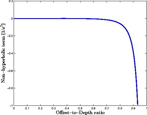

The coefficient c₃ is the term in the total traveltime function that controls the non-hyperbolicity characteristic for PS reflections. Figure  plots equation , as a function of the offset-to-depth ratio. Notice that the non-hyperbolicity is primarily observed for large values of the offset-to-depth ratio, this conclusion validates the assumption of Tessmer and Behle (1988), that is the non-hyperbolic moveout can be approximated with a hyperbola for small values of the offset-to-depth ratio. Also, note that the correction is always negative and ignoring it will result in overestimates values for the velocities.

Substituting equations , and into the total traveltime equation , I obtain the non-hyperbolic moveout equation for PS data  

$$t^2 = t_0^2 + \frac{x^2}{v_{\rm eff}^2} + \frac{x^4}{t_0^2 v... ...)}{4 \left( \gamma^{1/2} + \gamma^{-1/2} \right ) ^4} \right ].$$ (9)

Equation  depends only on two parameters: 1) the effective velocity ($v_{\rm eff}$), and 2) the P-to-S velocity ratio ($\gamma$). It is also important to note that this equation assumes a constant value of $\gamma$ in all layers. For the non-physical case of v_p=v_s, i.e. no converted waves, $\gamma$ equals 1, and equation () reduces to the conventional hyperbolic normal moveout equation. This equation also assumes a single layer model.

Figure  shows the traveltime computed with equation , with a constant P-velocity of 2 km/s, and S-velocity of 0.6 km/s, a maximum absolute offset of 7 km, and four horizontal reflectors at depths of 0.8, 1.5, 2.2, 2.9 km. The dotted curve represents non-hyperbolic moveout, equation (), and the solid curve represents the hyperbolic moveout equation, that is omitting the third term in equation (). Observe that for deeper reflectors and small offset both curves match reasonably well.

 

nhnmo Figure 2 Non-hyperbolic traveltime comparison with the hyperbolic approximation.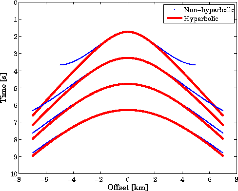

 

• Synthetic example