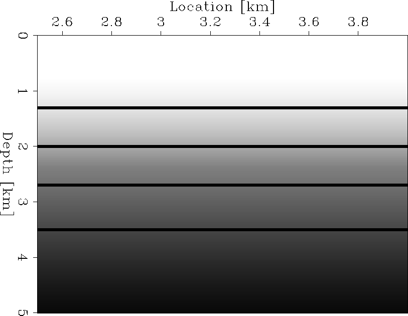
![[*]](http://sepwww.stanford.edu/latex2html/cross_ref_motif.gif) displays a simple synthetic model.
The model consists of four horizontal layers embedded in a vertical gradient
velocity model. The initial P-velocity is 2 km/s with a vertical-gradient
of 0.4
displays a simple synthetic model.
The model consists of four horizontal layers embedded in a vertical gradient
velocity model. The initial P-velocity is 2 km/s with a vertical-gradient
of 0.4
Figure ![[*]](http://sepwww.stanford.edu/latex2html/cross_ref_motif.gif) displays a simple synthetic model.
The model consists of four horizontal layers embedded in a vertical gradient
velocity model. The initial P-velocity is 2 km/s with a vertical-gradient
of 0.4
displays a simple synthetic model.
The model consists of four horizontal layers embedded in a vertical gradient
velocity model. The initial P-velocity is 2 km/s with a vertical-gradient
of 0.4 ![]() , and the initial S-velocity is 1 km/s
with a vertical gradient of 0.2
, and the initial S-velocity is 1 km/s
with a vertical gradient of 0.2 ![]() ; therefore, this
example has a constant P-to-S velocity ratio of
; therefore, this
example has a constant P-to-S velocity ratio of ![]() .
.
 |
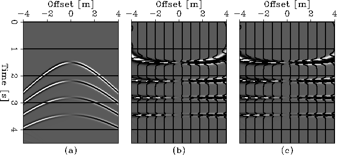
Figure ![[*]](http://sepwww.stanford.edu/latex2html/cross_ref_motif.gif) shows the results for this
experiment. Panel (a) exhibits the synthetic CMP gather.
Panel (b) shows the same CMP gather as in the previous
panel after hyperbolic NMO, that is using two terms in
the total traveltime equation. Panel (c) shows the same
CMP gather as in panel (a) after non-hyperbolic NMO, that
is using three terms in the total traveltime equation.
shows the results for this
experiment. Panel (a) exhibits the synthetic CMP gather.
Panel (b) shows the same CMP gather as in the previous
panel after hyperbolic NMO, that is using two terms in
the total traveltime equation. Panel (c) shows the same
CMP gather as in panel (a) after non-hyperbolic NMO, that
is using three terms in the total traveltime equation.
I use a Kirchhoff modeling scheme to obtain the synthetic data in panel (a). Observe the change in the polarity along the four reflections at zero offset. This polarity flip is characteristics of converted-wave data, since the P-to-S velocity ratio is constant then the polarity flip happens at zero offset.
Compare the results in panels (b) and (c). The hyperbolic normal moveout result, panel (b), presents an overcorrection for the the first reflection, that is visible at large offset values. This overcorrection is less severe after using non-hyperbolic moveout correction. However, the overcorrection caused by hyperbolic solution disappears after the third reflector, the hyperbolic moveout correction and the non-hyperbolic moveout equation achieve the same result for deep reflectors and short offset.
This simple example shows that for large offset-to-depth ratio more terms in the total traveltime equation yield better flat results are achieved. Also, for small offset-to-depth ratio both approximations achieved the same result; therefore, it is possible to still hyperbolic moveout equation to obtain a simple model of the Earth's subsurface.
 |
![[*]](http://sepwww.stanford.edu/latex2html/movie.gif)