


The transformation to the angle domain of PS-SODCIGs follows an approach similar
to the 2-D isotropic single-mode (PP) method Sava and Fomel (2003).
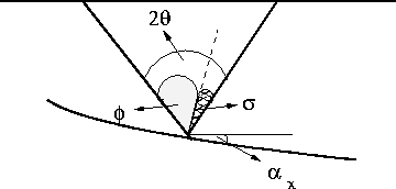
Figure ![[*]](http://sepwww.stanford.edu/latex2html/cross_ref_motif.gif) describes the angles I use in this section.
For the converted-mode case, I define
the following angles:
describes the angles I use in this section.
For the converted-mode case, I define
the following angles:
 |
||
| (31) |
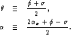
In definition the angles ![]() ,
, ![]() , and
, and
![]() represent the incident, reflected, and geological dip angles, respectively.
This definition is consistent with the single-mode case;
notice that for the single-mode case
the angles
represent the incident, reflected, and geological dip angles, respectively.
This definition is consistent with the single-mode case;
notice that for the single-mode case
the angles ![]() and
and ![]() are the same. Therefore,
the angle
are the same. Therefore,
the angle ![]() represents the reflection angle, and the
angle
represents the reflection angle, and the
angle ![]() represents the geological dip Biondi and Symes (2004); Sava and Fomel (2003).
For the converted-mode case, the angles
represents the geological dip Biondi and Symes (2004); Sava and Fomel (2003).
For the converted-mode case, the angles ![]() and
and ![]() are not the same.
Hence, the angle
are not the same.
Hence, the angle ![]() is the
half-aperture angle, and the angle
is the
half-aperture angle, and the angle ![]() is the pseudo-geological dip.
is the pseudo-geological dip.
 |

Throughout this chapter, I present a relationship between the known quantities from
our image, ![]() , and the half-aperture angle (
, and the half-aperture angle (![]() ).
Appendix A presents the full derivation of this relationship. Here, I present only
the final result, its explanation and its implications.
The final relationship to obtain converted-mode angle-domain common-image
gathers is the following (Appendix A):
).
Appendix A presents the full derivation of this relationship. Here, I present only
the final result, its explanation and its implications.
The final relationship to obtain converted-mode angle-domain common-image
gathers is the following (Appendix A):
| |
(32) |
 |
||
Equation consists of three main components. First ![]() is the
P-to-S velocity ratio. Next,
is the
P-to-S velocity ratio. Next, ![]() is the pseudo-opening angle.
This pseudo-opening angle is the
angle obtained throughout the conventional method to transform
SODCIGs into isotropic ADCIGs as described by Sava and Fomel (2003). Finally,
is the pseudo-opening angle.
This pseudo-opening angle is the
angle obtained throughout the conventional method to transform
SODCIGs into isotropic ADCIGs as described by Sava and Fomel (2003). Finally,
![]() is the field of local image-dips.
Equation describes the transformation from
the subsurface-offset domain
into the angle-domain for converted-wave data.
This equation is valid under the assumption of constant velocity. However, it
remains valid in a differential sense in an arbitrary velocity medium, by
considering that
is the field of local image-dips.
Equation describes the transformation from
the subsurface-offset domain
into the angle-domain for converted-wave data.
This equation is valid under the assumption of constant velocity. However, it
remains valid in a differential sense in an arbitrary velocity medium, by
considering that ![]() is the subsurface half-offset. Therefore, the limitation of
constant velocity applies in the neighborhood of the image. For
is the subsurface half-offset. Therefore, the limitation of
constant velocity applies in the neighborhood of the image. For ![]() ,
it is important to consider that every point of the image
is related to a point on the velocity model with the same image coordinates.
Notice that for the non-physical case of vp = vs, i.e. no converted waves,
,
it is important to consider that every point of the image
is related to a point on the velocity model with the same image coordinates.
Notice that for the non-physical case of vp = vs, i.e. no converted waves, ![]() ,and the angles
,and the angles ![]() and
and ![]() are the same.
are the same.