Methodology

I present a method to implement equations -. First, I describe the method and then illustrate it with a simple synthetic example. Throughout this section, I will refer to two different methods: first, the conventional method, and second, the proposed method. The conventional method consists of the transformation from SODCIGs into ADCIGs as in the single-mode case Sava and Fomel (2003). Figure  presents the flow chart for the proposed method.

 

flowADCIG
Figure 2 Flow chart to transform the subsurface-offset common-image gathers into the angle domain. The flow diagram also presents the mapping into P-ADCIGs and S-ADCIGs.

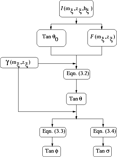The flow in Figure  presents the basic steps to implement and obtain the true angle-domain common-image gathers for converted-wave data (PS-ADCIGs). First, I use the final image, $I(m_{\xi},z_{\xi},h_{\xi})$, to obtain two main pieces of information: first, the pseudo-opening angle gathers, $\tan{\theta_0}$, using for example, the Fourier-domain approach Sava and Fomel (2003); second, the estimated image dip, $\d$, using plane-wave destructors Fomel (2002). For the second step, I combine $\tan{\theta_0}$ and $\d$ together with the $\gamma({\bf m_{\xi}})$-field using equation  to obtain true converted-wave angle-domain common-image gathers. Finally, I map these PS angle-domain common-image gathers into both the P-ADCIGs and the S-ADCIGs through equations  and , respectively.

 

ps-all-new
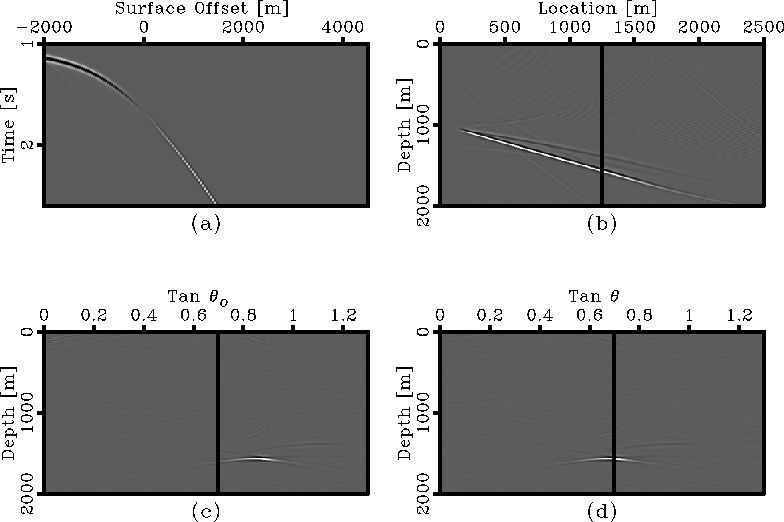Figure 3 Synthetic example that illustrates the method in Figure . Panel (a) is a single shot gather for a $30^\circ$ dipping layer event. Panel (b) is the image of this single shot gather. Panel (c) is the pseudo-opening angle, $\tan{\theta_0}$.Panel (d) is the true PS-ADCIG.

A simple synthetic example illustrates the flow in Figure . The synthetic dataset consists of a single shot experiment over a $30^\circ$ dipping layer. Panel (a) on Figure  shows the shot gather; observe that the top of the hyperbola is not at zero offset because of the reflector dip, and the polarity flip does not happen at the top of the hyperbola. Panel (b) shows the image of the single shot gather, which represents $I(m_{\xi},z_{\xi},h_{\xi})$ in the flow chart of Figure . The solid line in panel (b) represents the location for the CIG in study.

For this experiment the shot location is at 500 m, with the common image gather at 1000 m, and the geometry given for the reflector, the half aperture angle should be $35^\circ$. This corresponds to a value of $\tan\theta \approx 0.7$, that is represented with a solid line on both common image gathers at the bottom of Figure .

The angle-domain common-image gather in panel (c) of Figure  was obtained with the conventional method. Observe that the angle obtained is not the correct one. This ADCIG represents the tangent of the pseudo-opening angle, $\tan{\theta_0}$,of flow . The ADCIG in panel (c) combined with the dip information, $\d$,and the $\gamma({\bf m_{\xi}})$-field, results in the true PS-ADCIG. Panel (d) presents the result of this process. Notice the angle in the true PS-ADCIG coincides with the correct angle.

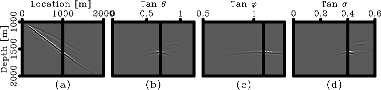
The last step for the flow chart in Figure  correspond to map the true PS-ADCIG into both a P-ADCIG and an S-ADCIG, each one corresponding to the P-incidence ($\phi$) and S-reflection ($\sigma$) angles, respectively. Figure  shows the result for this transformation. Panel (a) is the same image for the single shot gather on a $30^\circ$ dipping layer. Panel (b) is the corresponding true PS-ADCIG, which is taken at the location marked in the image. Panels (c) and (d) present the PS-ADCIG map into both the P-ADCIG and the S-ADCIG, respectively. Both angle gathers are obtained using equations  and  respectively.

As in the previous experiment, the computed value for the P-incidence angle is $47^\circ$, which corresponds to $\tan \phi\approx 1.09$. The computed value for the S-reflection angle is $22^\circ$, which corresponds to $\tan \sigma\approx 0.4$. Both of these values are represented by the solid lines in each of the three angle-domain common-image gathers on Figure .

 

ps-ind-new
Figure 4 Synthetic example that illustrates the last step of the method on Figure . Panel (a) is the image of a single shot gather on a $30^\circ$ dipping layer. Panel (b) is the true PS-ADCIG taken at the location of 1000 m. Panels (c) and (d) are the P-and-S ADCIGs, respectively.