Randomly dipping layers

On a horizontally layered earth, a common shotpoint gather looks like a common midpoint gather. For an earth model of random dipping planes the two kinds of gathers have quite different traveltime curves as we see in Figure 12.

 

randip
Figure 12 Seismic arrival times on an earth of random dipping planes. Left is for CSP. Right is for CMP.

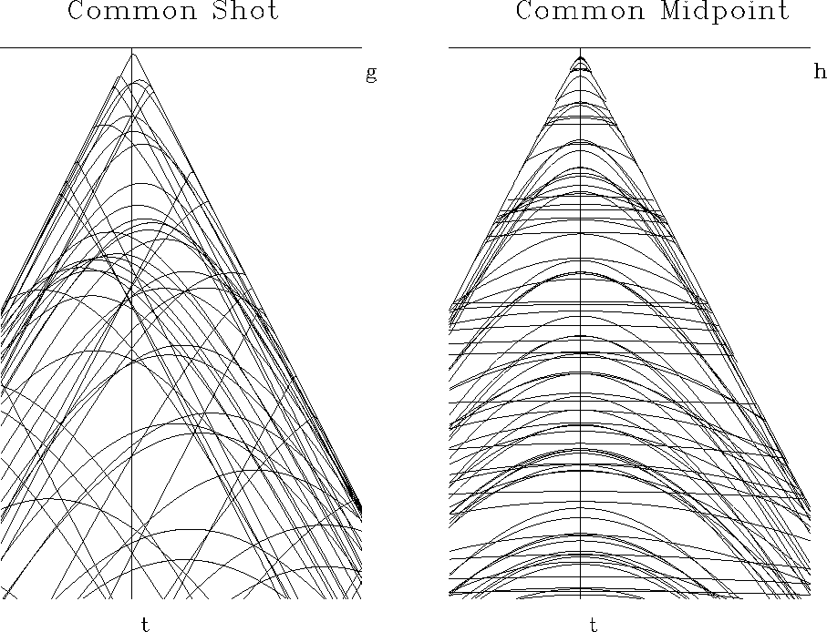
The common-shot gather is more easily understood. Although a reflector is dipping, a spherical wave incident remains a spherical wave after reflection. The center of the reflected wave sphere is called the image point. The traveltime equation is again a cone centered at the image point. The traveltime curves are simply hyperbolas topped above the image point having the usual asymptotic slope. The new feature introduced by dip is that the hyperbola is laterally shifted which implies arrivals before the fastest possible straight-line arrivals at vt = |g|. Such arrivals cannot happen. These hyperbolas must be truncated where vt = |g|. This discontinuity has the physical meaning of a dipping bed hitting the surface at geophone location |g|=vt. Beyond the truncation, either the shot or the receiver has gone beyond the intersection. Eventually both are beyond. When either is beyond the intersection, there are no reflections.

On the common-midpoint gather we see hyperbolas all topping at zero offset, but with asymptotic velocities higher (by the Levin cosine of dip) than the earth velocity. Hyperbolas truncate, now at |h| = tv/2, again where a dipping bed hits the surface at a geophone.

On a CMP gather, some hyperbolas may seem high velocity, but it is the dip, not the earth velocity itself that causes it. Imagine Figure 12 with all layers at $90^\circ$ dip (abandon curves and keep straight lines). Such dip is like the backscattered groundroll seen on the common-shot gather of Figure 9. The backscattered groundroll becomes a ``flat top'' on the CMP gather in Figure 12.

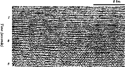
Such strong horizontal events near zero offset will match any velocity, particularly higher velocities such as primaries. Unfortunately such noise events thus make a strong contribution to a CMP stack. Let us see how these flat-tops in offset create the diagonal streaks you see in midpoint in Figure 13.

 

shelikof
Figure 13 CDP stack with water noise from the Shelikof Strait, Alaska. (by permission from Geophysics, Larner et al.[1983])

Consider 360 rocks of random sizes scattered in an exact circle of 2 km diameter on the ocean floor. The rocks are distributed along one degree intervals. Our survey ship sails from south to north towing a streamer across the exact center of the circle, coincidentally crossing directly over rock number 180 and number 0. Let us consider the common midpoint gather corresponding to the midpoint in the center of the circle. Rocks 0 and 180 produce flat-top hyperbolas. The top is flat for 0<|h|<1 km. Rocks 90 and 270 are $90^\circ$ out of the plane of the survey. Rays to those rocks propagate entirely within the water layer. Since this is a homogeneous media, the travel time expression of these rocks is a simple hyperbola of water velocity. Now our CMP gather at the circle center has a ``flat top'' and a simple hyperbola both going through zero offset at time t=2/v (diameter 2 km, water velocity). Both curves have the same water velocity asymptote and of course the curves are tangent at zero offset.

Now consider all the other rocks. They give curves inbetween the simple water hyperbola and the flat top. Near zero offset, these curves range in apparant velocity between water velocity and infinity. One of these curves will have an apparant velocity that matches that of sediment velocity. This rock (and all those near the same azimuth) will have velocities that are near the sediment velocity. This noise will stack very well. The CDP stack at sediment velocity will stack in a lot of water borne noise. This noise is propagating somewhat off the survey line but not very far off it.

Now let us think about the appearance of the CDP stack. We turn attention from offset to midpoint. The easiest way to imagine the CDP stack is to imagine the zero-offset section. Every rock has a water velocity asymptote. These asymptotes are evident on the CDP stack in Figure 13. This result was first recognized by Ken Larner.

Thus, backscattered low-velocity noises have a way of showing up on higher-velocity stacked data. There are two approaches to suppressing this noise: (1) mute the inner traces, and as we will see, (2) dip moveout processing.