Earth surface boundary condition

The program that created Figure 2 begins with an initial condition along the top boundary, and then this initial wavefield is extrapolated downward. So, the first question is: what is the mathematical function of x that describes a collapsing spherical (actually cylindrical) wave? An expanding spherical wave has an equation $\exp[-i\omega (t - r/v)]$,where the radial distance is $r=\sqrt{(x-x_0)^2+(z-z_0)^2}$ from the source. For a collapsing spherical wave we need $\exp[-i\omega (t + r/v)]$.Parenthetically, I'll add that the theoretical solutions are not really these, but something more like these divided by $\sqrt{r}$;actually they should be a Hankel functions, but the picture is hardly different when the exact initial condition is used. If you have been following this analysis, you should have little difficulty changing the initial conditions in the program to create the downgoing plane wave shown in Figure 3.

 

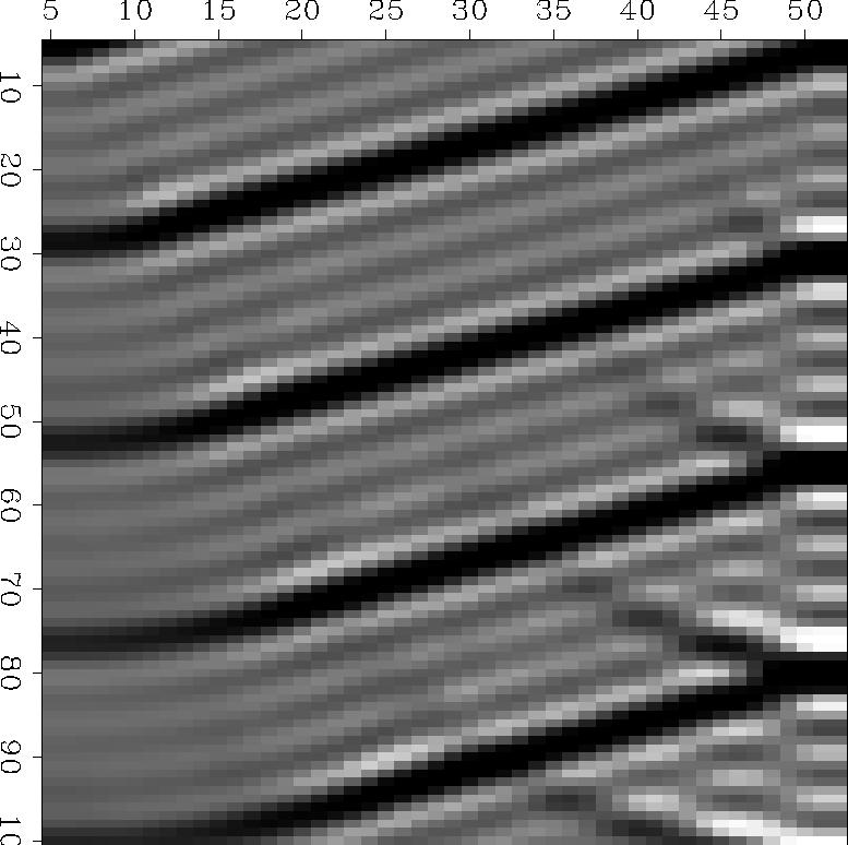
Mdipplane90 Figure 3 Specify program changes that give an initial plane wave propagating downward at an angle of 15$^\circ$ to the right of vertical. (Movie)

Notice the weakened waves in the zone of theoretical shadow that appear to arise from a point source on the top corner of the plot. You have probably learned in physics classes of ``standing waves''. This is what you will see near the reflecting side boundary if you recompute the plot with a single frequency nw=1. Then the plot will acquire a ``checkerboard'' appearance near the reflecting boundary. Even this figure with nw=4 shows the tendency.