 |
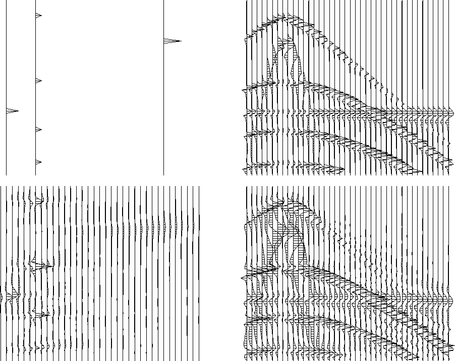
Figure 17 Top left: Slowness model. Top right: Data derived from it using the pseudounitary scale factor. Bottom left: the velocity spectrum of top right. Bottom right: data made from velocity spectrum.
 |
Figure 17 shows that on a second pass, the velocity spectrum of the slow wave is much smoothed. This suggests that it might be more efficient to parameterize the data with slowness squared rather than slowness itself. Another interesting thing about using slowness squared as an independent variable is that when slowness squared is negative (velocity imaginary) the data is matched by ellipses curving up instead of hyperbolas curving down.
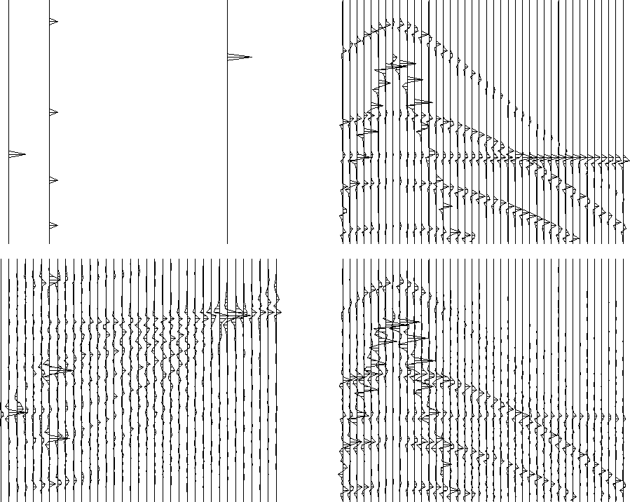 |
Figure 18 shows the effect of no antialiasing in either the field recording or the processing. The velocity spectrum is as sharp, if not sharper, but it is marred by a large amount of low-level noise.
Aliased data gives an interesting question. Should we use an aliased operator as in Figure 18 or should we use an antialiased operator as that in Figure 17? Figure 19 shows the resulting velocity analysis. The antialiased operator seems well worth while, even when applied to aliased data.
|
adataavel
Figure 19 Aliased data analyzed with antialiased operator. Compare to the lower left of Figure 18. | 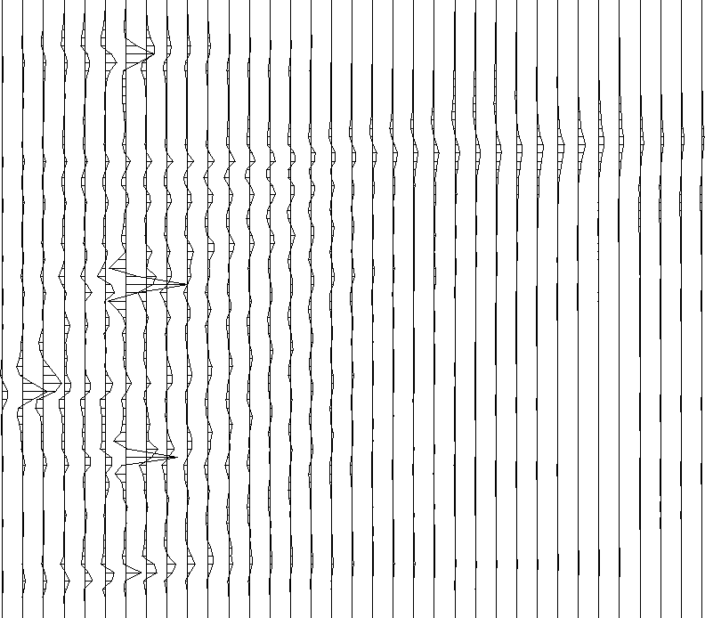 |
In real life, the field arrays are not ``dynamic'' (able to respond with space and time variable s0) but the data processing can be dynamic. Fourier and finite-difference methods of wave propagation and data processing are generally immune to aliasing difficulties. On the other hand, dynamic arrays in the data processing are a helpful feature of the ray approach whose counterparts seem unknown with Fourier and finite-difference techniques.
Since ![]() does not appear in physical modeling,
people are sometimes hesitant to put it in the velocity analysis.
If
does not appear in physical modeling,
people are sometimes hesitant to put it in the velocity analysis.
If ![]() is omitted from the modeling,
then |sx| should be put in the velocity analysis.
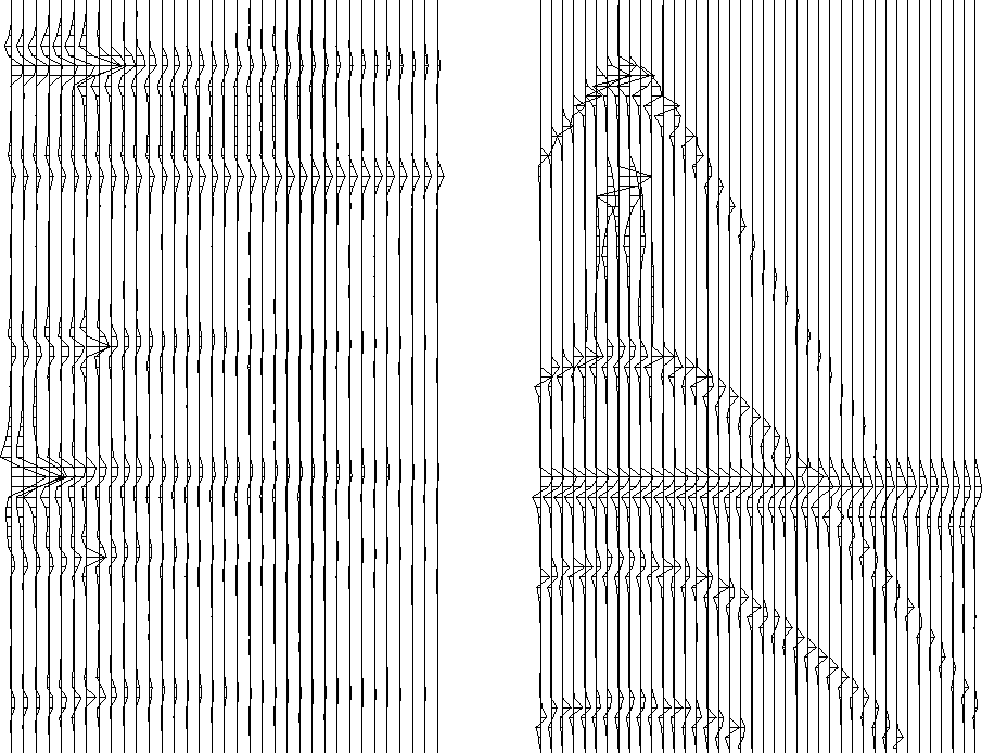
Failing to do so will give a result like in figure 20.
The principal feature of such a velocity analysis
is the velocity smearing.
A reason for smearing is that the zero-offset signal
is strong in all velocities.
Multiplying by
is omitted from the modeling,
then |sx| should be put in the velocity analysis.
Failing to do so will give a result like in figure 20.
The principal feature of such a velocity analysis
is the velocity smearing.
A reason for smearing is that the zero-offset signal
is strong in all velocities.
Multiplying by ![]() kills that signal
(which is never recorded in the field anyway).
The conceptual advantage of a pseudounitary transformation
like Figure 17 is that points in velocity space
are orthogonal components like Fourier components
whereas for nonunitary transforms
like with Figure 20
the different points in velocity space
are not orthogonal components.
kills that signal
(which is never recorded in the field anyway).
The conceptual advantage of a pseudounitary transformation
like Figure 17 is that points in velocity space
are orthogonal components like Fourier components
whereas for nonunitary transforms
like with Figure 20
the different points in velocity space
are not orthogonal components.
 |
Subroutine veltran() does the work.
# veltran -- velocity transform with anti-aliasing and sqrt(-i omega)
#
subroutine veltran(adj,add,psun,s02,anti,t0,dt,x0,dx,s0,ds,nt,nx,ns,model,data)
integer it,ix,is,  adj,add,psun,                           nt,nx,ns
real x, s, wt,               s02,anti,t0,dt,x0,dx,s0,ds,model(nt,ns),data(nt,nx)
temporary real slow(nt), half(nt,nx)
call null(               half,nt*nx)
call adjnull(      adj,add,                             model,nt*ns, data,nt*nx)
if( adj != 0)   do ix = 1, nx
                        call halfdifa( adj,   0, nt, half(1, ix), data(1, ix) )
do is= 1, ns {  s = s0 + (is-1) * ds;   do it=1,nt { slow(it) = s}
do ix= 1, nx {  x = x0 + (ix-1) * dx
        if     ( psun == 2 ) {  wt =       abs( s * x)  }       # vel tran
        else if( psun == 1 ) {  wt = sqrt( abs( s * x)) }       # pseudounitary
        else                 {  wt = 1.                 }       # modeling
        call trimo( adj, 1, t0,dt,dx, x, nt,slow, s02, _
                        wt , anti,  model(1,is),  half(1,ix))
        }}
if( adj == 0)   do ix = 1, nx
                        call halfdifa( adj, add, nt, half(1, ix), data(1, ix) )
return; end
![[*]](http://sepwww.stanford.edu/latex2html/cross_ref_motif.gif) be replaced by nearest-neighbor interpolation?
be replaced by nearest-neighbor interpolation?