


Next: TIME-STATISTICAL RESOLUTION
Up: Resolution
Previous: Resolution
The famous ``uncertainty principle'' of quantum mechanics resulted from
observations that subatomic particles behave like waves with wave
frequency proportional to particle momentum.
The classical laws of mechanics enable prediction
of the future of a mechanical system by
extrapolation from presently known position and momentum.
But because of the
wave nature of matter with momentum proportional to frequency,
such prediction requires simultaneous knowledge
of both the location and the frequency of a wave.
A sinusoidal wave has a perfectly clearly determined frequency,
but it is spread over the infinitely long time axis.
At the other extreme is a delta function,
which is nicely compressed to a point on
the time axis but contains a mixture of all frequencies.
A mathematical analysis of the uncertainty principle
is thus an analysis relating functions
to their Fourier transforms.
Such an analysis begins by definitions of time duration and spectral bandwidth.
The time duration of a damped exponential function is infinite if by
duration you mean the span of nonzero function values.
However,
for nearly all
practical purposes the time span is chosen as the time required for the
amplitude to decay to e-1 of its original value.
For many functions
the span is defined by the span between points on the time or frequency
axis where the curve (or its envelope) drop to half of the maximum value.
The
main idea is that the time span  or the frequency span
  should be able to include most of the total energy but need not contain
all of it.
The precise definition of and is
somewhat arbitrary and may be chosen to simplify analysis.
The general
statement is that for any function the time duration and the
spectral bandwidth are related by
should be able to include most of the total energy but need not contain
all of it.
The precise definition of and is
somewhat arbitrary and may be chosen to simplify analysis.
The general
statement is that for any function the time duration and the
spectral bandwidth are related by
| 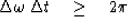 |
(1) |
Although it is easy to verify (1) in many special cases,
it is not very easy to deduce (1) as a general principle.
This has,
however, been done by D. Gabor.
He chose to define and by second moments.
A similar and perhaps more basic concept than the product of time and
frequency spreads is the relationship between spectral bandwidth
and rise time of a system response function.
The rise time of a system response is also defined somewhat arbitrarily,
often as the time
span between the time of excitation and the time at which the system
response is half its ultimate value.
In principle, a broad frequency
response can result from a rapid decay time as well as from a rapid
rise time.
Tightness in the inequality (1) may be associated
with situations in which a certain rise time is quickly
followed by an equal decay time.
Slackness in the inequality
(1) may be associated with increasing inequality between rise
time and decay time.
Slackness could also result from other combinations
of rises and falls such as random combinations.
Many systems respond very
rapidly compared to the rate at which they subsequently decay.
Focusing
our attention on such systems,
we can now seek to derive the inequality
(1) applied to rise time and bandwidth.
The first step is to choose
a definition for rise time.
The choice is determined not only for clarity and usefulness
but also by the need to ensure tractability of the subsequent analysis.
I have found a reasonable definition of rise time to be
| 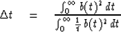 |
(2) |
where b(t) is the response function under consideration.
The numerator is just a normalizing factor.
The denominator says we have defined by the first negative moment.
For example,
if b(t) is a step function,
then the denominator integral diverges,
giving the desired  rise time.
If b(t)2 grows linearly from zero to t0 and then vanishes,
the rise time is t0/2,
again a reasonable definition.
rise time.
If b(t)2 grows linearly from zero to t0 and then vanishes,
the rise time is t0/2,
again a reasonable definition.
Although the Z transform method is a great aid in studying situations where
divergence (as 1/t) plays a key role,
it does have the disadvantage that it destroys the formal identity
between the time domain and the frequency domain.
Presumably this disadvantage is not fundamental since we can always
go to a limiting process in which the discretized time domain tends to a
continuum.
In order to utilize the analytic simplicity of the Z transform
we now consider the dual to the rise-time problem.
Instead of a time function
whose square vanishes identically at negative time we now consider a spectrum
 which vanishes at negative frequencies.
We measure how fast this spectrum can rise after
which vanishes at negative frequencies.
We measure how fast this spectrum can rise after  .We will find this to
be related to the time duration of the complex time function bt.
More precisely, we will now define the lowest significant frequency
component
.We will find this to
be related to the time duration of the complex time function bt.
More precisely, we will now define the lowest significant frequency
component  in the spectrum analogously to
(2) to be
in the spectrum analogously to
(2) to be
| 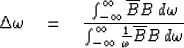 |
(3) |
Without loss of generality we can assume that the spectrum has been normalized
so that the numerator integral is unity.
In other words,
the zero lag of the auto-correlation of bt is +1.
Then
| 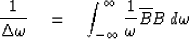 |
(4) |
Now we recall the bilinear transform which gives us various Z transform
expressions for  .The one we ordinarily use is the
integral
.The one we ordinarily use is the
integral  .The pole right on the unit circle at Z = 1 causes some nonuniqueness.
Because
.The pole right on the unit circle at Z = 1 causes some nonuniqueness.
Because  is an imaginary odd frequency function
we will take the desired expansion to be the odd function of time given by
is an imaginary odd frequency function
we will take the desired expansion to be the odd function of time given by
|  |
(5) |
Converting (4) to an integral on the unit circle in Z transform
notation we have
| 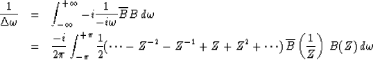 |
|
| (6) |
But since this integral selects
the coefficient of Z0 of its argument we have
| ![\begin{displaymath}
{1 \over \Delta \omega} \eq {-i \over 2} \left[ (r_{-1} - r_1) + (r_{-2} -r_2)
+ \cdots \right]\end{displaymath}](img24.gif) |
(7) |
where rt is the autocorrelation function of bt.
This may be further expressed as
| 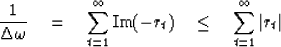 |
(8) |
The sum in (8) is like an integral representing area under the
|rt| function.
Imagine the |rt| function replaced by a rectangle function
of equal area.
This would define a  for the |rt| function.
Any autocorrelation function satisfies |rt| < r0 and we have
normalized r0 = 1.
Thus, we extend the inequality (8) by
for the |rt| function.
Any autocorrelation function satisfies |rt| < r0 and we have
normalized r0 = 1.
Thus, we extend the inequality (8) by
| 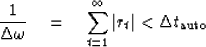 |
(9) |
Finally, we must relate the duration of a time function to the
duration of its autocorrelation .Generally speaking,
it is easy to find a long time function which has short autocorrelation.
Just take an arbitrary short time function
and convolve it by a long and tortuous all-pass filter.
The new function is long, but its autocorrelation is short.
If a time function has n nonzero points,
then its autocorrelation has only 2n -1 nonzero points.
It is obviously impossible to get a long autocorrelation function
out of a short time function.
It is not even fair to say that the autocorrelation
must lie under some tapering function.
To construct a time function with as long an autocorrelation as possible,
the best thing to do is to concentrate the energy in two lumps,
one at each end of the time function.
Even from this extreme example,
we see that it is not unreasonable to assert that
|  |
(10) |
inserting into (9) we have the uncertainty relation
|  |
(11) |
The more usual form of the uncertainty principle uses the frequency
variable  and a different definition of , namely
time duration rather than rise time. It is
and a different definition of , namely
time duration rather than rise time. It is
|  |
(12) |
The choice of a  scaling factor to convert rise time to
duration is indicative of the approximate nature of the inequalities.
scaling factor to convert rise time to
duration is indicative of the approximate nature of the inequalities.
EXERCISES:
- Consider B(Z) = [1 - (Z/Z0)n]/(1 -Z/Z0) in the limit Z0 goes to
the unit circle.
Sketch the time function and its squared amplitude.
Sketch the frequency function and its squared amplitude.
Choose
 and .
and . - A time series made up of two frequencies may be written as

Given  ,
,  , b0, b1, b2, b3 show how to calculate
the amplitude and phase angles of the two sinusoidal components.
, b0, b1, b2, b3 show how to calculate
the amplitude and phase angles of the two sinusoidal components.
- Consider the frequency function graphed below.
E4-1-3
Figure 1 Exercise 4.1.3.
|
| 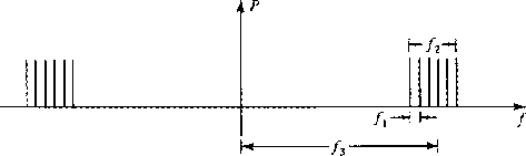 |

Describe the time function in rough terms indicating the times corresponding to
1/f1, 1/f2, 1/f3.
Try to avoid algebraic calculation.
Sketch an approximate result.
PROBLEM FOR RESEARCH
Can you find a method of defining and of one-sided
wavelets in such a way that for minimum-phase wavelets only the uncertainty
principle takes on the equality sign?
Next: TIME-STATISTICAL RESOLUTION
Up: Resolution
Previous: Resolution
Stanford Exploration Project
10/30/1997