


Next: About this document ...
Up: Matrices and multichannel time
Previous: MATRIX FILTERS, SPECTRA, AND
A Markov process is another mathematical model for a time series.
Until now it has found little use in geophysics,
but we will include it anyway
because it might become useful
and it is easily explained with the methods previously developed.
Suppose that xt could take on only integer values.
A given value is called a state.
As time proceeds,
transitions are made from the jth state
to the ith state according to a probability matrix pij.
The system has no memory.
The next state is probabilistically dependent on the current state
but independent of the previous states.
The classic example is of a frog
in a lily pond.
As time goes by, the frog jumps from one lily pad to another.
He may be more likely to jump to a near one than to a far one.
The state of the system is the number of the pad the frog currently occupies.
The transitions are his jumps.
To begin with, one defines a state probability  ,the probability
that the system will occupy state i after k transitions if its state is
known at k = 0.
We also define the transition matrix Pij.
Then
,the probability
that the system will occupy state i after k transitions if its state is
known at k = 0.
We also define the transition matrix Pij.
Then
| 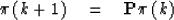 |
(44) |
The initial-state probability vector is  .Since the initial state is known,
then is all zeros except for a one (1) in the position
corresponding to the initial state.
For example, see the state-transition diagram of Figure 2.
.Since the initial state is known,
then is all zeros except for a one (1) in the position
corresponding to the initial state.
For example, see the state-transition diagram of Figure 2.
5-3
Figure 2 An example of a state-transition diagram.
|
| 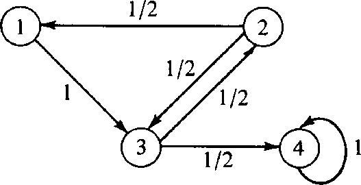 |

The diagram corresponds to the probability matrix
![\begin{displaymath}
\left[ \begin{array}
{c}
\pi_1 \\ \pi_2 \\ \pi_3 \\ \pi_4...
...{c}
\pi_1 \\ \pi_2 \\ \pi_3 \\ \pi_4 \end{array} \right]_{k}\end{displaymath}](img144.gif)
Since at each time a transition must occur,
we have that the sum of the elements in a column must be unity.
In other words,
the row vector ![$[1 \ \ 1 \ \ 1 \ \ 1]$](img145.gif) is an eigenvector of P with unit eigenvalue.
Let us define the Z transform of the probability vector as
is an eigenvector of P with unit eigenvalue.
Let us define the Z transform of the probability vector as
|  |
(45) |
In terms of Z transforms (44) becomes
| ![\begin{eqnarray}[\pi (1) + Z\pi(2) + \cdots ]
&= & {\bf P}[\pi(0) + Z\pi(1) + \c...
...(0) \nonumber \\ \Pi (Z) &= & ({\bf I} - Z{\bf P})^{-1}\, \pi (0)\end{eqnarray}](img147.gif) |
|
| |
| |
| (46) |
Thus we have expressed the general solution
to the problem as a function of the matrix
P times an initial-state vector.
There will be values of Z for which the inverse matrix
to  does not exist.
These values Zj are given by det
does not exist.
These values Zj are given by det or det
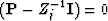 .Clearly the Z-1j are the eigenvalues of P.
Utilizing Sylvester's theorem, then, we have
.Clearly the Z-1j are the eigenvalues of P.
Utilizing Sylvester's theorem, then, we have
| 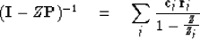 |
(47) |
Some modification to (47) is required
if there are repeated eigenvalues.
Equation (47) is essentially a partial fraction expansion.
A typical term has the form
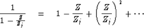
Thus coefficients at successive powers of Z decline with time in the form
(Z-1j)t.
It is clear that,
if probabilities are to be bounded,
the roots 1/Zj must be inside the unit circle (recall minimum phase).
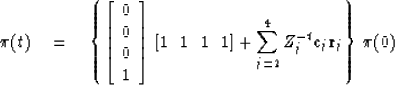
We have already shown that one the of the roots Z1 is always unity.
This leads to the ``steady-state'' solution 1t = 1.
In our particular example,
one can see by inspection that the steady-state probability
vector is ![$[0 \ \ 0 \ \ 0 \ \ 1]^T$](img153.gif) so the general solution is of the form
so the general solution is of the form
Finally, a word of caution must be added.
Occasionally defective matrices arise
(incomplete set of eigenvectors) and for these the Sylvester theorem
does not apply.
In such cases, the solutions turn out to contain not only
terms like Z-tj but also terms like tZ-t and t2 Z-t.
It is the same situation as that applying
to ordinary differential equations with constant coefficients.
Ordinarily, the solutions are of the form (ri)t
where ri is the ith root of the indicial equation but the presence
of repeated roots gives rise to solutions like trti.
Next: About this document ...
Up: Matrices and multichannel time
Previous: MATRIX FILTERS, SPECTRA, AND
Stanford Exploration Project
10/30/1997