Empty bins and inverse interpolation

 

Let us review the big picture. In Chapter we developed adjoints and in Chapter we developed inverse operators. Logically, correct solutions come only through inversion. Real life, however, seems nearly the opposite. This is puzzling but intriguing.

Every time you fill your car with gasoline, it derives much more from the adjoint than from inversion. I refer to the fact that ``practical seismic data processing'' relates much more to the use of adjoints than of inverses. It has been widely known for about the last 15 years that medical imaging and all basic image creation methods are like this. It might seem that an easy path to fame and profit would be to introduce the notion of inversion, but it is not that easy. Both cost and result quality enter the picture.

First consider cost. For simplicity, consider a data space with N values and a model (or image) space of the same size. The computational cost of applying a dense adjoint operator increases in direct proportion to the number of elements in the matrix, in this case N². To achieve the minimum discrepancy between theoretical data and observed data (inversion) theoretically requires N iterations raising the cost to N³.

Consider an image of size $m\times m=N$.Continuing, for simplicity, to assume a dense matrix of relations between model and data, the cost for the adjoint is m⁴ whereas the cost for inversion is m⁶. We'll consider computational costs for the year 2000, but noticing that costs go as the sixth power of the mesh size, the overall situation will not change much in the foreseeable future. Suppose you give a stiff workout to a powerful machine; you take an hour to invert a $4096\times 4096$ matrix. The solution, a vector of 4096 components could be laid into an image of size $64\times 64= 2^6\times 2^6 = 4096$.Here is what we are looking at for costs:

$$(m\times m )^2 (512\times 512)^2$$ adjoint cost (2⁹ 2⁹)² 2³⁶

$$(m\times m )^3 (64\times 64)^3$$ inverse cost (2⁶ 2⁶)³ 2³⁶

These numbers tell us that for applications with dense operators, the biggest images that we are likely to see coming from inversion methods are $64\times 64$ whereas those from adjoint methods are $512\times 512$.For comparison, the retina of your eye is comparable to your computer screen at $1000\times 1000$.We might summarize by saying that while adjoint methods are less than perfect, inverse methods are ``legally blind'' :-)

http://sepwww.stanford.edu/sep/jon/family/jos/gifmovie.html holds a movie blinking between Figures and .

 

512x512 Figure 1 Jos greets Andrew, ``Welcome back Andrew'' from the Peace Corps. At a resolution of 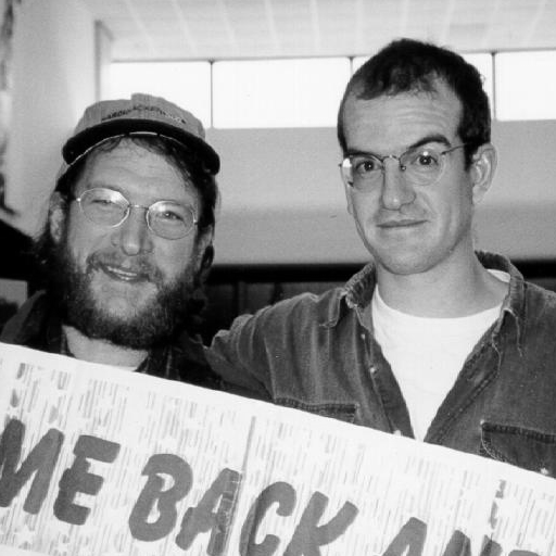$512\times 512$, this picture is about the same as the resolution as the paper it is printed on, or the same as your viewing screen, if you have scaled it to 50% of screen size.

 

64x64 Figure 2 Jos greets Andrew, ``Welcome back Andrew'' again. At a resolution of 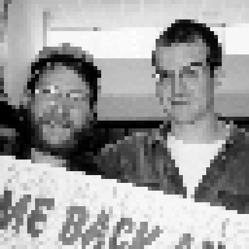$64\times 64$ the pixels are clearly visible. From far the pictures are the same. From near, examine their glasses.

This cost analysis is oversimplified in that most applications do not require dense operators. With sparse operators, the cost advantage of adjoints is even more pronounced since for adjoints, the cost savings of operator sparseness translate directly to real cost savings. The situation is less favorable and much more muddy for inversion. The reason that Chapter 2 covers iterative methods and neglects exact methods is that in practice iterative methods are not run to their theoretical completion but they run until we run out of patience.

Cost is a big part of the story, but the story has many other parts. Inversion, while being the only logical path to the best answer, is a path littered with pitfalls. The first pitfall is that the data is rarely able to determine a complete solution reliably. Generally there are aspects of the image that are not learnable from the data.

In this chapter we study the simplest, most transparant example of data insufficiency. Data exists at irregularly spaced positions in a plane. We set up a cartesian mesh and we discover that some of the bins contain no data points. What then?