Seismic field data examples

Figures - are based on exploration seismic data from the Gulf of Mexico deep water. A ship carries an air gun and tows a streamer with some hundreds of geophones. First we look at a single pop of the gun. We use all the geophone signals to create a single 1-D PEF for the time axis. This changes the average temporal frequency spectrum as shown in Figure .

 

antoinedecon1
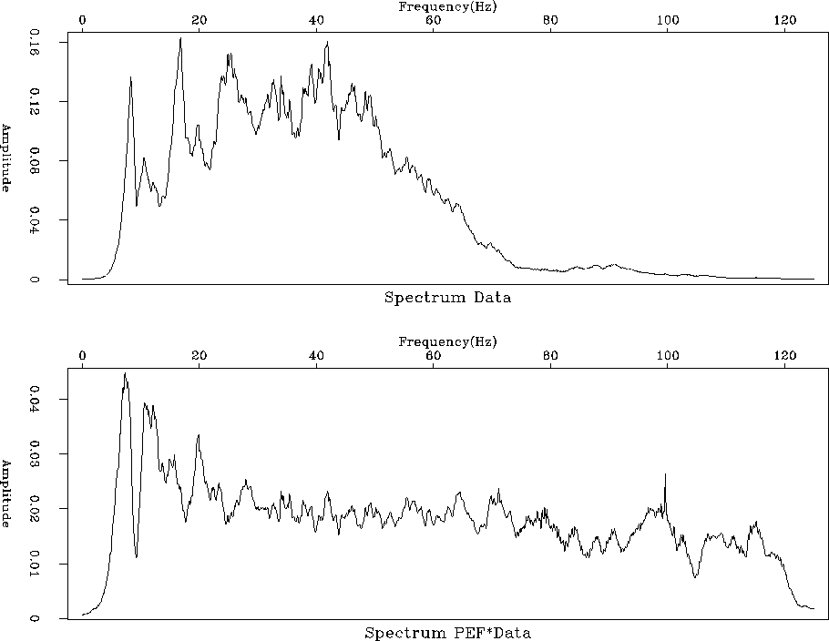Figure 10 $\omega$ spectrum of a shot gather of Figure  before and after 1-D decon with a 30 point filter.

Signals from 60 Hz to 120 Hz are boosted substantially. The raw data has evidently been prepared with strong filtering against signals below about 8 Hz. The PEF attempts to recover these signals, mostly unsuccessfully, but it does boost some energy near the 8 Hz cutoff. Choosing a longer filter would flatten the spectrum further. The big question is, ``Has the PEF improved the appearance of the data?''

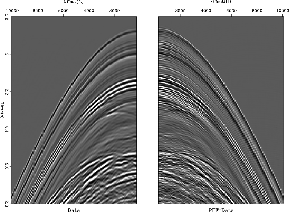
The data itself from the single pop, both before and after PE-filtering is shown in Figure . For reasons of esthetics of human perception I have chosen to display a mirror image of the PEF'ed data. To see a blink movie of superposition of before-and-after images you need the electronic book. We notice that signals of high temporal frequencies indeed have the expected hyperbolic behavior in space. Thus, these high-frequency signals are wavefields, not mere random noise.

 

antoinedecon
Figure 11 Raw data with its mirror. Mirror had 1-D PEF applied, 30 point filter.

Given that all visual (or audio) displays have a bounded range of amplitudes, increasing the frequency content (bandwidth) means that we will need to turn down the amplification so we do not wish to increase the bandwidth unless we are adding signal.

Increasing the spectral bandwidth always requires us to diminish the gain.

The same ideas but with a two-dimensional PEF are in Figure  (the same data but with more of it squeezed onto the page.) As usual, the raw data is dominated by events arriving later at greater distances. After the PEF, we tend to see equal energy in dips in all directions. We have strongly enhanced the ``backscattered'' energy, those events that arrive later at shorter distances.

 

antoinedecon2
Figure 12 A 2-D filter (here $20\times 5$) brings out the backscattered energy.

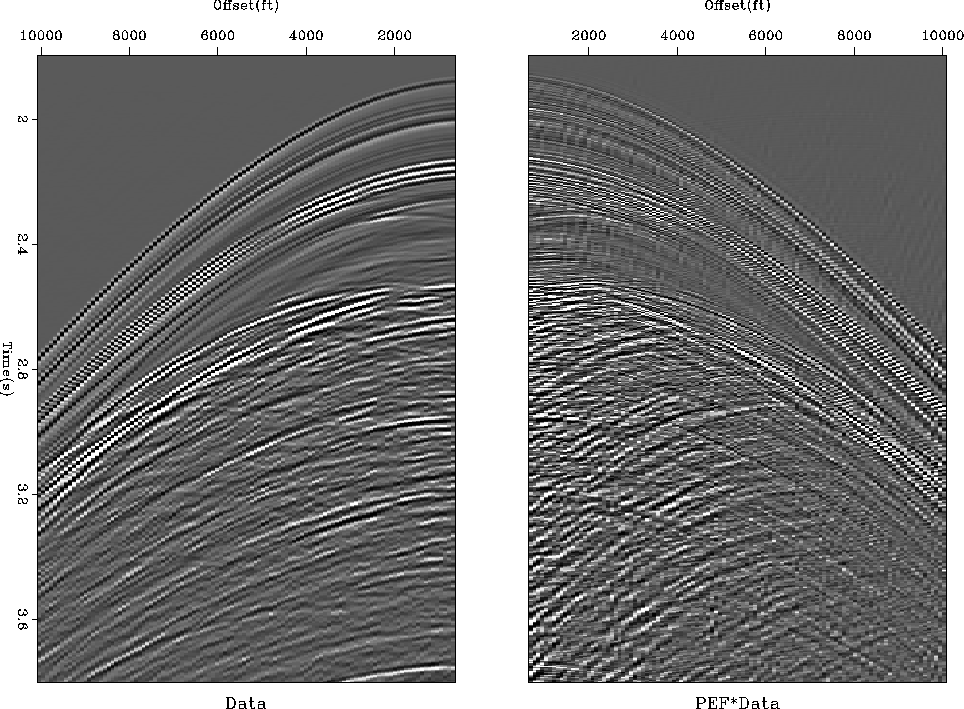Figure  shows echos from the all shots, the nearest receiver on each shot. This picture of the earth is called a ``near-trace section.'' This earth picture shows us why there is so much backscattered energy in Figure  (which is located at the left side of Figure ). The backscatter comes from any of the many of near-vertical faults.

We have been thinking of the PEF as a tool for shaping the spectrum of a display. But does it have a physical meaning? What might it be? Referring back to the beginning of the chapter we are inclined to regard the PEF as the convolution of the source waveform with some kind of water-bottom response. In Figure  we used many different shot-receiver separations. Since each different separation has a different response (due to differing moveouts) the water bottom reverberation might average out to be roughly an impulse. Figure  is a different story. Here for each shot location, the distance to the receiver is constant. Designing a single channel PEF we can expect the PEF to contain both the shot waveform and the water bottom layers because both are nearly identical in all the shots. We would rather have a PEF that represents only the shot waveform (and perhaps a radiation pattern).

 

antoinedecon3
Figure 13 Raw data, near-trace section (top). Filtered with a two-channel PEF (bottom). The movie has other shaped filters.

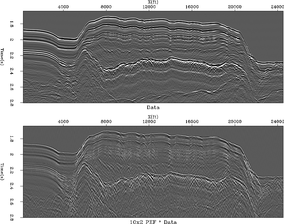Let us consider how we might work to push the water-bottom reverberation out of the PEF. This data is recorded in water 600 meters deep. A consequence is that the sea bottom is made of fine-grained sediments that settled very slowly and rather similarly from place to place. In shallow water the situation is different. The sands near estuaries are always shifting. Sedimentary layers thicken and thin. They are said to ``on-lap and off-lap.'' Here I do notice where the water bottom is sloped the layers do thin a little. To push the water bottom layers out of the PEF our idea is to base its calculation not on the raw data, but on the spatial prediction error of the raw data. On a perfectly layered earth a perfect spatial prediction error filter would zero all traces but the first one. Since a 2-D PEF includes spatial prediction as well as temporal prediction, we can expect it to contain much less of the sea-floor layers than the 1-D PEF. If you have access to the electronic book, you can blink the figure back and forth with various filter shapes.