Inversions with geostat

In geophysical estimation (inversion) we use model styling (regularization) to handle the portion of the model that is not determined by the data. This results in the addition of minimal noise. Alternately, like in Geostatistics, we could make an assumption of statistical stationarity and add much more noise so the signal variance in poorly determined regions matches that in well determined regions. Here is how to do this. Given the usual data fitting and model styling goals

$$\begin{eqnarray} \bold 0 &\approx& \bold L \bold m -\bold d \\ \bold 0 &\approx& \bold A \bold m\end{eqnarray}$$ (32) (33)

We introduce a sample of random noise $\bold n$ and fit instead these regressions

$$\begin{eqnarray} \bold 0 &\approx& \bold L \bold m -\bold d \\ \bold 0 &\approx& \bold A \bold m -\bold n\end{eqnarray}$$ (34) (35)

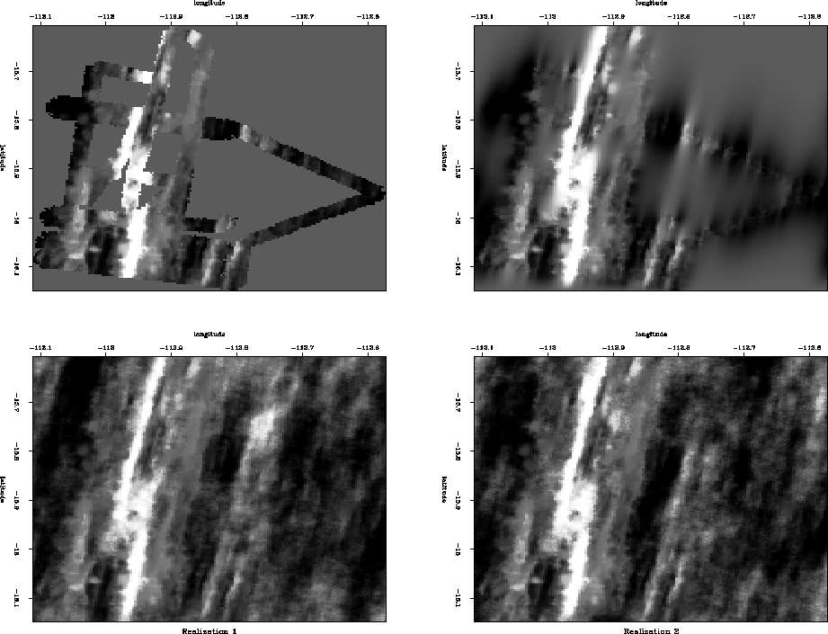
Of course you get a different solution for each different realization of the random noise. You also need to be a little careful to use noise $\bold n$of the appropriate variance. Figure shows a result on the SeaBeam data.

 

bobsea
Figure 20 Top left is binned data. Top right extends the data with a PEF. The bottom two panels add appropriately colored random noise in the regions of missing data.

Bob Clapp developed this idea at SEP and also applied it to interval velocity estimation, the example of Figures -.