|
subsine390
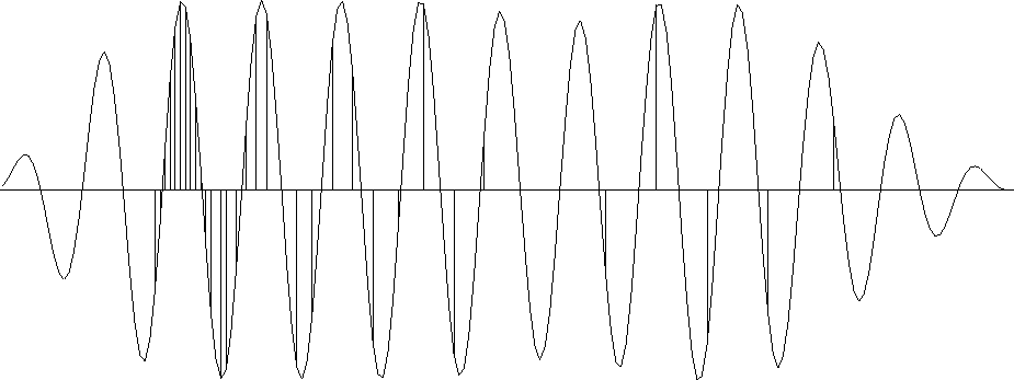
Figure 26 Interpolating with a three-term filter. The interpolated signal is fairly monofrequency. |  |
![[*]](http://sepwww.stanford.edu/latex2html/movie.gif)
![[*]](http://sepwww.stanford.edu/latex2html/cross_ref_motif.gif) and
and ![[*]](http://sepwww.stanford.edu/latex2html/cross_ref_motif.gif) show the same example as in Figures
show the same example as in Figures
![[*]](http://sepwww.stanford.edu/latex2html/cross_ref_motif.gif) and
and
![[*]](http://sepwww.stanford.edu/latex2html/cross_ref_motif.gif) .
What is new here is that the proper PEF
is not given but is determined from the data.
Figure
.
What is new here is that the proper PEF
is not given but is determined from the data.
Figure ![[*]](http://sepwww.stanford.edu/latex2html/cross_ref_motif.gif) was made with a three-coefficient filter (1,a1,a2) and
Figure
was made with a three-coefficient filter (1,a1,a2) and
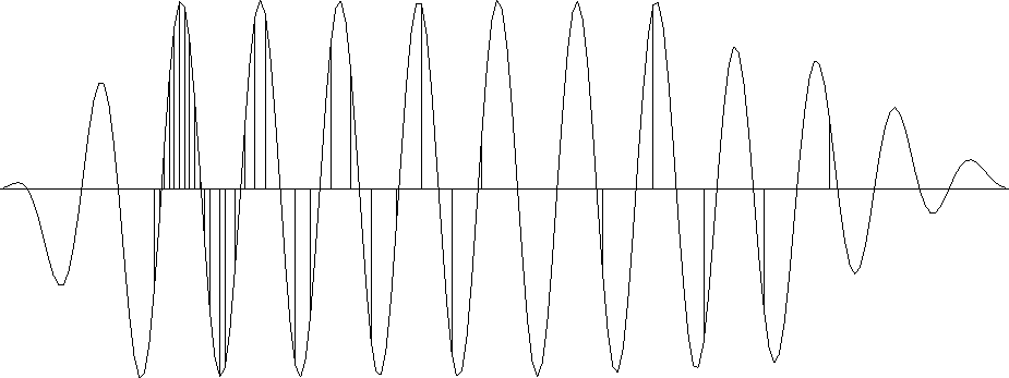
Figure ![[*]](http://sepwww.stanford.edu/latex2html/cross_ref_motif.gif) was made with a five-coefficient filter
(1,a1,a2,a3,a4).
The main difference in the figures is where the data is sparse.
The data points in Figures
was made with a five-coefficient filter
(1,a1,a2,a3,a4).
The main difference in the figures is where the data is sparse.
The data points in Figures
![[*]](http://sepwww.stanford.edu/latex2html/cross_ref_motif.gif) ,
,
![[*]](http://sepwww.stanford.edu/latex2html/cross_ref_motif.gif) and
and
![[*]](http://sepwww.stanford.edu/latex2html/cross_ref_motif.gif) are samples from a sinusoid.
are samples from a sinusoid.
|
subsine390
Figure 26 Interpolating with a three-term filter. The interpolated signal is fairly monofrequency. |  |
![[*]](http://sepwww.stanford.edu/latex2html/movie.gif)
|
subsine590
Figure 27 Interpolating with a five term filter. |  |
![[*]](http://sepwww.stanford.edu/latex2html/movie.gif)
|
Comparing Figures
|