


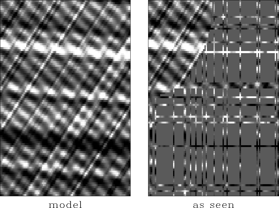
![[*]](http://sepwww.stanford.edu/latex2html/cross_ref_motif.gif) shows an example of sparse tracks;
it is not realistic
in the upper-left corner
(where it will be used for testing),
in a quarter-circular disk where
the data covers the model densely.
Such a dense region is ideal for determining the 2-D PEF.
Indeed, we cannot
determine a 2-D PEF from the sparse data lines,
because at any place you put the filter
(unless there are enough adjacent data lines),
unknown filter coefficients will multiply missing data.
So every fitting goal is nonlinear
and hence abandoned by the algorithm.
shows an example of sparse tracks;
it is not realistic
in the upper-left corner
(where it will be used for testing),
in a quarter-circular disk where
the data covers the model densely.
Such a dense region is ideal for determining the 2-D PEF.
Indeed, we cannot
determine a 2-D PEF from the sparse data lines,
because at any place you put the filter
(unless there are enough adjacent data lines),
unknown filter coefficients will multiply missing data.
So every fitting goal is nonlinear
and hence abandoned by the algorithm.
 |


The set of test data shown in Figure
is a superposition of three functions like plane waves.
One plane wave looks like low-frequency horizontal layers.
Notice that the various layers vary in strength with depth.
The second wave is dipping about ![]() down to the right
and its waveform is perfectly sinusoidal.
The third wave dips down
down to the right
and its waveform is perfectly sinusoidal.
The third wave dips down ![]() to the left
and its waveform is bandpassed random noise like the horizontal beds.
These waves will be handled differently by different processing schemes,
so I hope you can identify all three.
If you have difficulty,
view the figure at a grazing angle from various directions.
to the left
and its waveform is bandpassed random noise like the horizontal beds.
These waves will be handled differently by different processing schemes,
so I hope you can identify all three.
If you have difficulty,
view the figure at a grazing angle from various directions.
Later we will make use of the dense data region,
but first let ![]() be the east-west PE operator
and
be the east-west PE operator
and ![]() be the north-south operator
and let the signal or image be
be the north-south operator
and let the signal or image be ![]() .The fitting residuals are
.The fitting residuals are
 |
(19) |
Figure shows
the result of using a single one-dimensional PEF
along either the vertical or the horizontal axis.
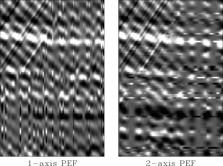 |
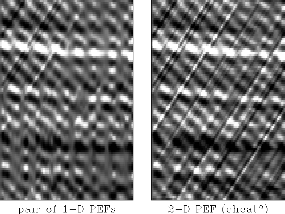
Figure compares
the use of a pair of 1-D PEFs versus a single 2-D PEF
(which needs the ``cheat'' corner in Figure .
 |
![[*]](http://sepwww.stanford.edu/latex2html/movie.gif)
Studying Figure we conclude
(what theory predicts) that