Wide-angle wave extrapolation

Let $s = - i \hat \omega$ denote the causal, positive, discrete representation of the differentiation operator, say,  

$$s \eq - i\, \hat \omega \eq {2 \over \Delta t} \ { 1 \ -\ \rho Z \over 1 \ +\ \rho Z }$$ (61)

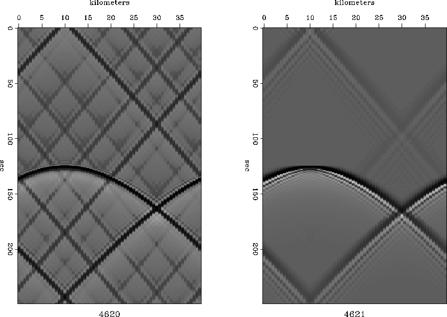
Figure 6 compares hyperbolas constructed with $\omega$ to those constructed with $\hat \omega$.

 

cxfreq
Figure 6 Hyperbolas with real frequency (left) and complex frequency (right). (Plotting uses square root gain described in chapter ).

You see a pleasing drop in wraparound noise. It seems to work better than the $\epsilon$ in chapter . As we will see, the introduction of complex-valued $\hat \omega$ leads to a more natural handling of the square root at the evanescent transition.

Consider the following recursion starting from R₀ = s:  

$$R_{n+1} \eq s\ +\ { X^2 \over s \ +\ R_n }$$ (62)

This recursion produces continued fractions. Francis Muir introduced it as a means of developing wide-angle square-root approximations for migration (chapter ). and he developed his three rules to show that every R_n is an impedance function. To see why every R_n is an impedance function, first note that the denominator s + R_n is, for n=0, the sum of two impedance functions. Then its inverse is an impedance function, and multiplication by the real positive constant X² and addition of another s both preserve the properties of impedance functions. Recursively we see that all the R_n are impedances.

As N becomes large this recursion either converges or it does not. Supposing that it does, we can see what it will converge to by setting $R_{n+1} = R_n = R_{\infty} = R$.Thus,

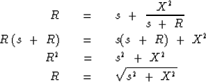$$\begin{eqnarray} R \ \ \ &=&\ \ \ s \ +\ { X^2 \over s \ +\ R } \\ R \ (s\ +\ R)... ...\ &=&\ \ \ s^2 \ +\ X^2 \\ R \ \ \ &=&\ \ \ \sqrt { s^2 \ +\ X^2 }\end{eqnarray}$$ (63) (64) (65) (66)

In wave-extrapolation problems X² is $v^2 \ k_x^2$, where v is the wave velocity and k_x is the horizontal spatial frequency, namely, the Fourier dual to the horizontal x-axis. Performing these substitutions we have  

$$R \eq \pm \sqrt { - {\hat \omega}^2 \ +\ v^2 \, k_x^2 }$$ (67)

So R is like $\pm i k_z v$.Remember that R₀, the first approximation to R, is $-i \hat \omega$.So downgoing waves are  

$$D(x,z,t) \eq D(x,0,t) \ \ e^{ i k_x x}\ e^{ -\,R\,z/v } \ e^{ - i \omega t }$$ (68)

To switch from downgoing to upcoming waves, we could either change the sign in front of R or we take the complex conjugate of R. The difference is what you want to do with the real part--do you want the wave to grow or not? Consider the dissipation of waves in the exploding reflector model. They damp as they propagate from the explosion to the surface. This means that as we migrate them, they should be exponentially growing. But we don't really want that. We really want to assure that they are not growing, perhaps we even want them decaying as we extrapolate them back. So for migration we downward continue monochromatic waves with  

$$U(x,z,t) \eq U(x,0,t) \ \ e^{ i k_x x}\ e^{ - \bar R \,z/v } \ e^{ - i \omega t }$$ (69)

although the real behavior of a wave from an exploding reflector wave would be  

$$U(x,z,t) \eq U(x,0,t) \ \ e^{ i k_x x}\ e^{ +\,R\,z/v } \ e^{ - i \omega t }$$ (70)

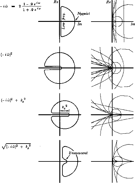
To examine the phase of the complex quantity R, set v=1 obtaining  

$$R \eq \sqrt {(- \, i \hat \omega )^2 \ +\ k_x^2 }$$ (71)

First note that $( - \, i \hat \omega )$ is causal because of its Z-transform representation. By squaring the Z-transform we see that $( - \, i \hat \omega )^2$ is also causal. In the time domain, k_x² is a delta function at the time origin. Thus R² given by (71) is causal. Figure 7 shows how the phase of (71) is constructed from its constituents. To illustrate the behavior of $-i \hat \omega$ from zero to infinity, I include both an artist's conception and the function on itself, overlain at various magnifications. The function $-i \hat \omega$ is a periodic with $\omega$ and its real and imaginary parts plot to a closed curve. To show the rate of change of the function, I sampled $\omega$ at 2$^\circ$ intervals. From great distance the function is a circle. Close up it looks like a line parallel to the imaginary axis.

R² is causal and from Figure 7 we can see that it has a ``branch cut'' property. That is, the phase of R has the positive real property. Theorem 5 forces R to be causal and minimum phase. That, with the phase defined by Figure 7, proves that R, given by (71), is an impedance function.

 

kzplane
Figure 7 Complex plane diagram of constituents of the extrapolation operator R given by equation (71). The center column shows an artist's conception. The right column shows the function at several magnifications simultaneously.