


The double-square-root equation is
| |
(72) |

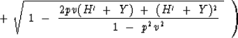 |
(73) |
Equation (73) is an exact representation of the double-square-root equation in what is called retarded Snell midpoint coordinates.
The coordinate system (58), (59), (60), and (61) can describe any wavefield in any medium. It is is particularly advantageous, however, only in stratified media of velocity near v(z) for rays that are roughly parallel to any ray with the chosen Snell parameter p. There is little reason to use these coordinates unless they ``fit'' the wave being studied. Waves that fit are those that are near the chosen p value. This means that H' doesn't get too big. A variety of simplifying expansions of (73) are possible. There are many permutations of magnitude inequalities among the three ingredients pv, H', and Y. You will choose the expansion according to the circumstances. The appropriate expansions and production considerations, however, have not yet been fully delineated. But let us take a look at two possibilities.
First, any dataset can be decomposed by stepout into many datasets, each with a narrow bandwidth in stepout space--CMP slant stacks, for example. For any of these datasets, H' could be ignored altogether. Then (73) would reduce to
 |
(74) |
| |
(75) |
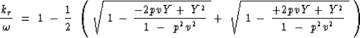
Next, let us make up an approximation to (73) which is separable in Y and H'. Equation (75) provides the first part. Then take Y=0 and keep all terms up to quadratics in H':
| |
(76) |
A separable approximation of (73) is (75) plus (76). It is no accident that there are no linear powers of H' in (76). The coordinate system was designed so that energy near the chosen model Y=0 and H=pv should not drift in the (h' , t' )-plane as the downward continuation proceeds.
The velocity spectrum idea represented by equation (76) is to use the H' term to focus the data on the (h' ,t' )-plane. After focusing, it should be possible to read interval velocities directly as slopes connecting events on the gathers. This approach was used in the dissertation of Alfonso Gonzalez [1982].