


Ordinarily we regard a common-midpoint gather as a collection of seismic traces, that is, a collection of time functions, each one for some particular offset h. But this (h,t) data space could be represented in a different coordinate system. A system with some nice attributes is the radial-trace system introduced by Turhan Taner. In this system the traces are not taken at constant h, but at constant angle. The idea is illustrated in Figure 17.
|
otto
Figure 17 Inside the data volume of a reflection seismic traverse are planes called radial-trace sections. A point scatterer inside the earth puts a hyperbola on a radial-trace section. | 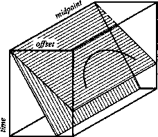 |

Besides having some theoretical advantages, which will become apparent, this system also has some practical advantages, notably: (1) the traces neatly fill the space where data is nonzero; (2) the traces are close together at early times where wavelengths are short, and wider apart where wavelengths are long; and (3) the energy on a given trace tends to represent wave propagation at a fixed angle. The last characteristic is especially important with multiple reflections. But for our purposes the best attribute of radial traces is still another one.
Richard Ottolini noticed that a point scatterer in the earth appears on a radial-trace section as an exact hyperbola, not a flat-topped hyperboloid. The travel-time curve for a point scatterer, Cheops' pyramid, can be written as a ``string length'' equation, or a stretched-circle equation. Making the definition
| |
(13) |
![[*]](http://sepwww.stanford.edu/latex2html/cross_ref_motif.gif) )
yields
)
yields
| |
(14) |
 |
We will see that the radial hyperbola of Figure 18
is easier to handle than
the flat-topped hyperboloid that is seen at constant h.
Refer to the equations in Table 7.2.
| migration | ||
| zero-offset diff. | ||
| DMO+NMO | ||
| radial DMO | ||
| radial NMO | ||
The second equation in Table 7.2 is the usual exploding reflector
equation for zero-offset migration.
It may also be obtained from the DSR by setting ![]() .As written it contains the earth velocity,
not the half velocity.
Equation (14) says that hyperbolas of differing
.As written it contains the earth velocity,
not the half velocity.
Equation (14) says that hyperbolas of differing ![]() values
are related to one another by scaling the z-axis by
values
are related to one another by scaling the z-axis by ![]() .According to Fourier transform theory,
scaling z by a
.According to Fourier transform theory,
scaling z by a ![]() divisor will
scale kz by a
divisor will
scale kz by a ![]() multiplier.
This means the first equation in Table 7.2 can be used for migrating
and diffracting hyperbolas on radial-trace sections.
Eliminating kz from
the first and second equations yields
the middle equation
multiplier.
This means the first equation in Table 7.2 can be used for migrating
and diffracting hyperbolas on radial-trace sections.
Eliminating kz from
the first and second equations yields
the middle equation ![]() in Table 7.2.
This middle equation combines the operation of migrating all
offsets (really any radial angle) and then diffracting out to zero offset.
Thus the total effect is that of offset continuation ,
i.e. NMO and DMO.
The last two equations in Table 7.2 are a decomposition of the middle
equation
in Table 7.2.
This middle equation combines the operation of migrating all
offsets (really any radial angle) and then diffracting out to zero offset.
Thus the total effect is that of offset continuation ,
i.e. NMO and DMO.
The last two equations in Table 7.2 are a decomposition of the middle
equation ![]() into two sequential
processes,
into two sequential
processes, ![]() and
and ![]() .These two processes are like DMO and NMO, but the operations
occur in radial space.
Radial NMO is a simple time-invariant s tretch; hence
the notation
.These two processes are like DMO and NMO, but the operations
occur in radial space.
Radial NMO is a simple time-invariant s tretch; hence
the notation ![]() .
.
Unlike the constant-offset case, dip moveout is now done before the stretching, velocity-estimating step. Let us confirm that the dip moveout is truly velocity-independent. Substitute (13) into the radial DMO transformation in Table 7.2 to get the equation for transformation from time to stretched time:
| |
(15) |
The dip-moveout process, ![]() ,can be conveniently implemented
with a Stolt-type algorithm using (15).
,can be conveniently implemented
with a Stolt-type algorithm using (15).
The foregoing analysis has assumed a constant velocity. A useful practical approximation might be to revert to a v(z) analysis after the dip moveout, just before conventional velocity analysis, stack, and zero-offset migration.
Both the radial-trace method and Hale's constant-offset method handle all angles exactly in a constant-velocity medium, but neither method treats velocity stratification exactly nor is it clear that this can be done--since neither method is rooted in the DSR. Yilmaz [1979] rooted his DMO work in the DSR, so his method can be expected to be exact for velocity stratification, but Yilmaz could not avoid angle-dependent approximations. So there remains theoretical work to be done.