


The conjugate-gradient method is really a family of methods. Mathematically these algorithms all converge to the answer in n (or fewer) steps where there are n unknowns. But the various methods differ in numerical accuracy, treatment of underdetermined systems, accuracy in treating ill-conditioned systems, space requirements, and numbers of dot products. I will call the method I use in this book the ``book3'' method. I chose it for its clarity and flexibility. I caution you, however, that among the various CG algorithms, it may have the least desirable numerical properties.
The ``conjugate-gradient method'' was introduced by Hestenes and Stiefel in 1952. A popular reference book, ``Numerical Recipes,'' cites an algorithm that is useful when the weighting function does not factor. (Weighting functions are not easy to come up with in practice, and I have not found any examples of nonfactorable weighting functions yet.) A high-quality program with which my group has had good experience is the Paige and Saunders LSQR program. A derivative of the LSQR program has been provided by Nolet. A disadvantage of the book3 method is that it uses more auxiliary memory vectors than other methods. Also, you have to tell the book3 program how many iterations to make.
There are a number of nonlinear optimization codes that reduce to CG in the limit of a quadratic function.
According to Paige and Saunders,
accuracy can be lost by explicit use of vectors
of the form ![]() ,which is how the book3 method operates.
An algorithm with better numerical properties,
invented by Hestenes and Stiefel,
can be derived by algebraic rearrangement.
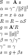
This rearrangement
(adapted from Paige and Saunders by Lin Zhang)
for the problem
,which is how the book3 method operates.
An algorithm with better numerical properties,
invented by Hestenes and Stiefel,
can be derived by algebraic rearrangement.
This rearrangement
(adapted from Paige and Saunders by Lin Zhang)
for the problem ![]() is
is
 |
||
A program that implements this algorithm in a manner consistent
with a blending of cgmeth() ![[*]](http://sepwww.stanford.edu/latex2html/cross_ref_motif.gif) and cgstep()
is hestenes().
and cgstep()
is hestenes().
subroutine hestenes( nx,x, nr,yy,rr, aaa, niter)
integer i, iter,     nx,   nr,            niter
real    alpha, beta, gamma, gammam
real    dot
real    x(nx), yy(nr), rr(nr), aaa(nr,nx)
temporary real g(nx), s(nx), ss(nr)
do i= 1, nx
        x(i) = 0.
do i= 1, nr
        rr(i) = yy(i)
call matmult( 1, aaa, nx,g, nr,yy)
do i= 1, nx
        s(i) = g(i)
gammam = dot(nx,g,g)
do iter= 0, niter {
        call matmult( 0, aaa, nx,s, nr,ss)
        alpha = gammam / dot(nr,ss,ss)
        do i = 1, nx
                x(i) = x(i) + alpha*s(i)
        do i = 1, nr
                rr(i) = rr(i) - alpha*ss(i)
        call matmult( 1, aaa, nx,g, nr,rr)
        gamma = dot(nx,g,g)
        beta = gamma / gammam
        gammam = gamma
        do i = 1, nx
                s(i) = g(i) + beta*s(i)
        }
return; end
I have not used the Hestenes and Stiefel version of the CG method
for the tutorial programs in this book
because
I wish to isolate features of geophysical analysis
from features of solution by the CG method.
The blending of geophysical features
with solution details
is worsened by the combination of Fortran and
this improved version of the CG algorithm.