The prediction form of a two-dip filter

Now we handle two dips simultaneously. The following filter destroys a wave that is sloping down to the right:

$$\begin{array} {ccc} -1 &\cdot &\cdot \ \cdot &\cdot &1 \end{array}$$ (8)

The next filter destroys a wave that is sloping less steeply down to the left:

$$\begin{array} {cc} \cdot &-1 \ 1 &\cdot \end{array}$$ (9)

Convolving the above two filters together, we get  

$$\begin{array} {rrrr} \cdot & 1 &\cdot &\cdot \ -1 &\cdot &\cdot & -1 \ \cdot &\cdot & 1 &\cdot \end{array}$$ (10)

The 2-D filter (10) destroys waves of both slopes. Given appropriate interlacing, the filter (10) destroys the data in Figure 14 both before and after interpolation. To find filters such as (10), I adjust coefficients to minimize the power out of filters like

$$\begin{array} {ccccc} v & w & x & y & z \ a & b & c & d & e \ \cdot &\cdot & 1 &\cdot &\cdot \end{array}$$ (11)

A filter of this shape is suitable for figures like 14 and 15.

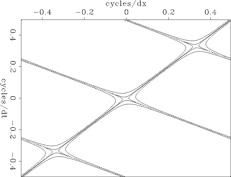
Let us examine the Fourier domain for this filter. The filter (10) was transformed to the Fourier domain; it was multiplied by its conjugate; the square root was taken; and contours are plotted at near-zero magnitudes in Figure 18. The slanting straight lines have slopes at the two dips that are destroyed by the filters. Noticing the broad lows where the null lines cross, we might expect to see energy at this temporal and spatial frequency, but I have not noticed any.

 

fk2dip Figure 18 Magnitude of two-dimensional Fourier transform of the 2-D filter contoured at .01 and at .1.

 

# CINJOF -- Convolution INternal with Jumps. Output and FILTER are adjoint.
#
subroutine cinjof( adj, add, jump,   n1,n2,xx, nb1,nb2,bb, yy)
integer            adj, add, jump,   n1,n2,    nb1,nb2    # jump subsamples data
real                                  xx( n1,n2),  bb( nb1,nb2),  yy( n1,n2)
integer y1,y2, x1,x2, b1, b2, ny1, ny2
call adjnull( adj, add,                            bb, nb1*nb2,   yy, n1*n2)
ny1 = n1 - (nb1-1) * jump;              if( ny1<1 ) call erexit('cinjof: ny1<1')
ny2 = n2 - (nb2-1);                     if( ny2<1 ) call erexit('cinjof: ny2<1')
if( adj == 0 )
        do b2=1,nb2 { do y2=1,ny2 {     x2 =  y2 - (b2-nb2)      
        do b1=1,nb1 { do y1=1,ny1 {     x1 =  y1 - (b1-nb1) * jump
                                yy(y1,y2) = yy(y1,y2) + bb(b1,b2) * xx(x1,x2)
                        }} }}
else
        do b2=1,nb2 { do y2=1,ny2 {     x2 =  y2 - (b2-nb2)      
        do b1=1,nb1 { do y1=1,ny1 {     x1 =  y1 - (b1-nb1) * jump
                                bb(b1,b2) = bb(b1,b2) + yy(y1,y2) * xx(x1,x2)
                        }} }}
return; end

In practice, wavefronts have curvature, so we will estimate the 2-D filters in many small windows on a wall of data. Therefore, to eliminate edge effects, I designed the 2-D filter programs starting from the 1-D internal convolution program convin() . The subroutine for two-dimensional filtering is cinjof() . The adjoint operation included in this subroutine is exactly what we need for estimating the filter.

A companion program, cinloi(), is essentially the same as cinjof(), except that in cinloi() the other adjoint is used (for unknown input instead of unknown filter), and there is no need to interlace the time axis. A new feature of cinloi() is that it arranges for the output residuals to come out directly on top of their appropriate location on the original data. In other words, the output of the filter is at the ``1.'' Although the edge conditions in this routine are confusing, it should be obvious that xx(,) is aligned with yy(,) at bb(lag1,lag2).

 

# CINLOI -- Convolution INternal with Lags.  Output is adjoint to INPUT.
#
subroutine cinloi( adj, add, lag1,lag2,nb1,nb2,bb,  n1,n2, xx, yy)
integer            adj, add, lag1,lag2,nb1,nb2,     n1,n2        # lag=1 causal
real                                    bb(nb1,nb2), xx(n1,n2), yy(n1,n2)
integer y1,y2, x1,x2, b1,b2
call adjnull(      adj, add,                         xx,n1*n2,  yy,n1*n2 )
if( adj == 0 )
        do b2=1,nb2 { do y2= 1+nb2-lag2, n2-lag2+1 {  x2= y2 - b2 + lag2      
        do b1=1,nb1 { do y1= 1+nb1-lag1, n1-lag1+1 {  x1= y1 - b1 + lag1      
                                yy(y1,y2) = yy(y1,y2) + bb(b1,b2) * xx(x1,x2)
                                }} }}
else
        do b2=1,nb2 { do y2= 1+nb2-lag2, n2-lag2+1 {  x2= y2 - b2 + lag2      
        do b1=1,nb1 { do y1= 1+nb1-lag1, n1-lag1+1 {  x1= y1 - b1 + lag1      
                                xx(x1,x2) = xx(x1,x2) + bb(b1,b2) * yy(y1,y2)
                                }} }}
return; end