


Letting n go to infinity
does not take us to the expectation ![]() .The problem is, as we increase n,
we increase the frequency resolution but not the statistical resolution
(i.e., the fluctuation around
.The problem is, as we increase n,
we increase the frequency resolution but not the statistical resolution
(i.e., the fluctuation around ![]() ).
To increase the statistical resolution,
we need to simulate ensemble averaging.
There are two ways to do this:
).
To increase the statistical resolution,
we need to simulate ensemble averaging.
There are two ways to do this:
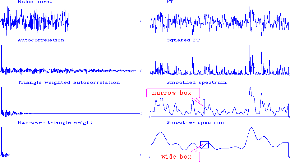 |

The second method is illustrated in Figure 10.
This figure shows a noise burst of 240 points.
Since the signal is even,
the burst is effectively 480 points wide,
so the autocorrelation is 480 points from center to end: the
number of samples will be the same for all cases.
The spectrum is very rough.
Multiplying the autocorrelation by a triangle function effectively
smooths the spectrum by a sinc-squared function, thus reducing the
spectral resolution (![]() ). Notice that
). Notice that ![]() is equal here to the width of the sinc-squared function, which is
inversely proportional to the length of the triangle (
is equal here to the width of the sinc-squared function, which is
inversely proportional to the length of the triangle (![]() ).
).
However, the first taper takes the autocorrelation width from 480 lags
to 120 lags.
Thus the spectral fluctuations ![]() should drop by a factor of 2,
since the count of terms sk in
should drop by a factor of 2,
since the count of terms sk in ![]() is
reduced to 120 lags.
The width of the next weighted autocorrelation
width is dropped from 480 to 30 lags.
Spectral roughness should consequently drop
by another factor of 2.
In all cases,
the average spectrum is unchanged,
since the first lag of the autocorrelations is unchanged.
This implies a reduction
in the relative spectral fluctuation proportional to the square root
of the length of the triangle (
is
reduced to 120 lags.
The width of the next weighted autocorrelation
width is dropped from 480 to 30 lags.
Spectral roughness should consequently drop
by another factor of 2.
In all cases,
the average spectrum is unchanged,
since the first lag of the autocorrelations is unchanged.
This implies a reduction
in the relative spectral fluctuation proportional to the square root
of the length of the triangle (![]() ).
).
Our conclusion follows:
|
The trade-off among resolutions of time, frequency, and spectral amplitude is
|