Numerical experiments

In the first example, we test our method on a constant velocity model(v=1km/s) with two-dimensional geometry $\{(x,z):-0.5\le x \le 0.5,0\le z \le 1.0\}$.

In this case, all the desired quantities have an obvious analytical solution to compare against the computed solutions. We compare the results obtained by two approaches, the first approach is computing all the quantities on the fixed output grid which reduces to be a first order method, the second is computing all the quantities by adaptive gridding. The ouput grid is $51\times 51$ with $\Delta{x}=\Delta{z}=0.02$. For adaptive grid, maxref is set to be 5 with the coarsest grid $17 \times 17$, and the error tolerance is set to be 0.0001.

Figures 1 and 2 show the traveltime contours by the two approaches, from which we cannot see any differences between two approaches. Similarly, we cannot see any differences in accuracy between two approaches from take-off angle, as shown in figures 3 and 4. This is due to visual limitations of graphics.

Figures 5 and 6 are contours of $\tau_{x}$ computed by two approaches. We can see that $\tau_{x}$ by the fixed grid approach is oscillating, but $\tau_{x}$ by the adaptive grid traveltime solver is convergent. Similar conclusions can be drawn for , as shown in figures 7 and 8.

Now we come to take-off angle derivatives. Figure 9 and 10 are contours of $\phi_{x}$ by two approaches. Because the coefficients in the advection equation for take-off angle depend on the traveltime gradient, any first order traveltime solver results in inaccurate $\nabla \tau$ which leads to the divergence of $\phi_{x}$, as shown in figure 9. However, the adaptive gridding approach gives us accurate traveltime gradients, which leads to the convergent $\phi_{x}$, as shown in figure 10. Similar conclusions can be drawn for $\phi_{z}$, as shown in figure 11 and 12.

To illustrate further the difference of accuracy between two approaches, figures 13 and 14 show the error distributions of $\phi_{x}$ and $\phi_{z}$.

Finally, the amplitudes based on the gradients of traveltime and take-off angle computed by the two approaches are shown in figures 15 and 16, one is divergent by the fixed grid approach, another accurate by the adaptive gridding approach.

In the second example, we use our new eikonal and amplitude solver in 2D Kirchhoff prestack migration and inversion. Figure 17 shows the impulse response by inversion with an ENO 3rd order eikonal solver. Figure 18 shows the impulse response by inversion with a WENO 5th order eikonal solver. By figures 17 and 18, we can see that the WENO 5th order solver does give us a more smooth amplitude than ENO 3rd solver.

 

comtau.fir Figure 1 Traveltime for constant velocity model: fixed grid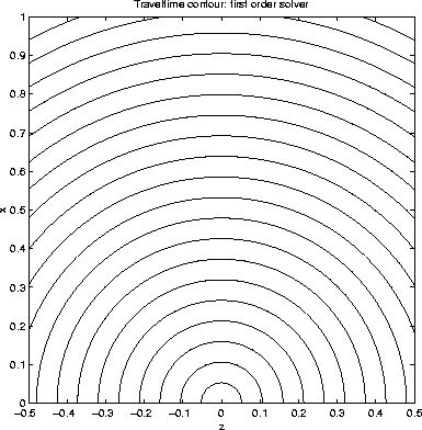

 

comtau.ada Figure 2 Traveltime for constant velocity model: adaptive grid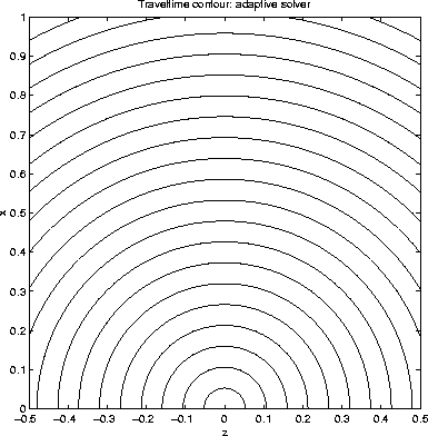

 

cometa.fir Figure 3 Take-off angle 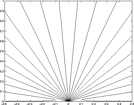$\phi$ for constant velocity model: fixed grid

 

cometa.ada Figure 4 Take-off angle 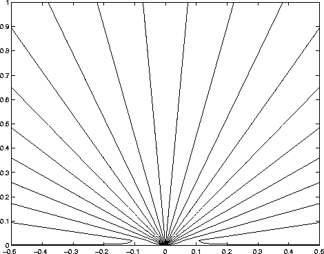$\phi$ for constant velocity model: adaptive grid

 

comtaux.fir Figure 5 Traveltime x derivative $\tau_{x}$ for constant velocity model: fixed grid

 

comtaux.ada Figure 6 Traveltime x derivative 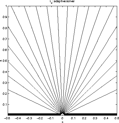$\tau_{x}$ for constant velocity model: adaptive grid

 

comtauz.fir Figure 7 Traveltime z derivative 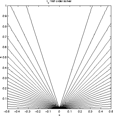$\tau_{z}$ for constant velocity model: fixed grid

 

comtauz.ada Figure 8 Traveltime z derivative $\tau_{z}$ for constant velocity model: adaptive grid

 

angxder.fir Figure 9 Take-off angle x derivative 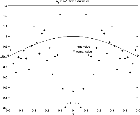$\phi_{x}$ at z=1 for constant velocity model: fixed grid

 

angxder.ada Figure 10 Take-off angle x derivative 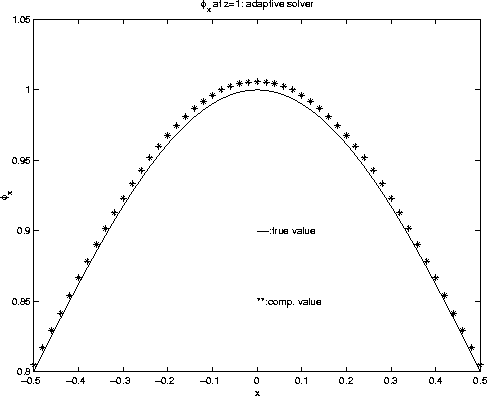$\phi_{x}$ at z=1 for constant velocity model: adaptive grid

 

angzder.fir Figure 11 Take-off angle z derivative 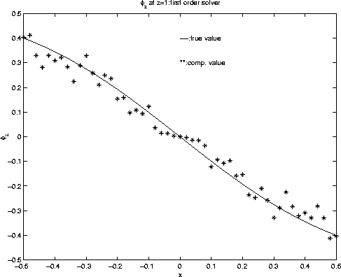$\phi_{z}$ at z=1 for constant velocity model: fixed grid

 

angzder.ada Figure 12 Take-off angle z derivative 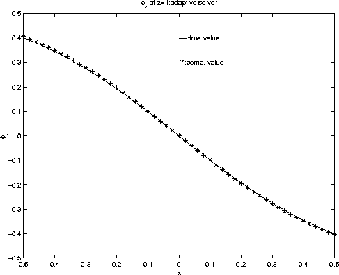$\phi_{z}$ at z=1 for constant velocity model: adaptive grid

 

angxzerr.fir Figure 13 Error distribution in take-off angle derivatives 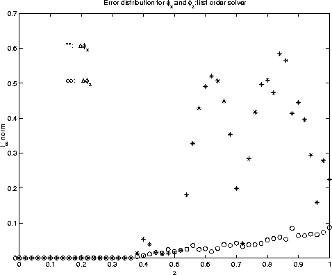$\phi_{x}$ and $\phi_{z}$: fixed grid

 

angxzerr.ada Figure 14 Error distribution in take-off angle derivatives 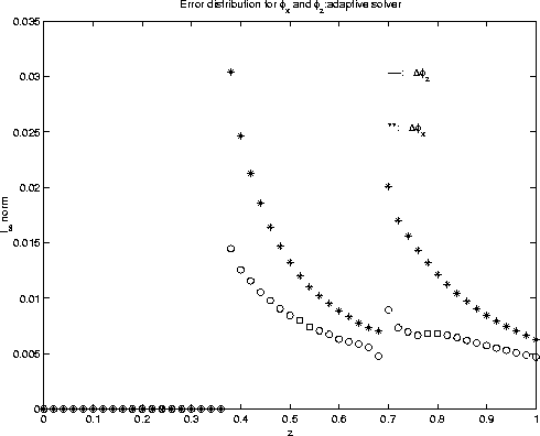$\phi_{x}$ and $\phi_{z}$: adaptive grid

 

amp.fir Figure 15 Amplitude for constant velocity model: fixed grid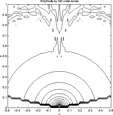

 

amp.ada Figure 16 Amplitude for constant velocity model: adaptive grid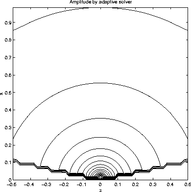

 

eno600.ada Figure 17 The impulse response by inversion with ENO 3rd order adaptive eikonal solver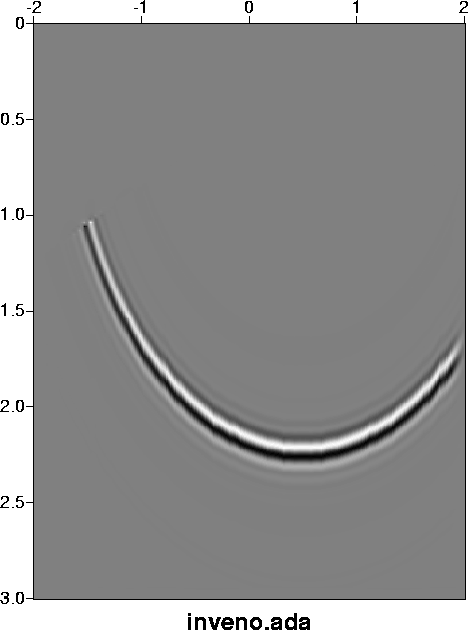

 

weno600.ada Figure 18 The impulse response by inversion with WENO 5th order adaptive eikonal solver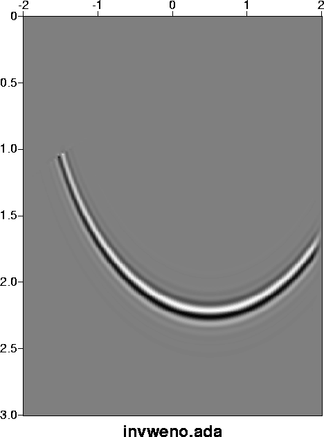