The inverse problem

Having defined the forward operator H and its adjoint ${\bf H}^ \dag$, we can now pose the inverse problem. Inverse theory helps us to find a velocity panel which synthesizes a given CMP gather via the operator H. In equations, given data d (CMP gather), we want to solve for the model m (velocity panel)

$$\bf{Hm}=\bf{d},$$

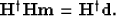
which is equivalent to the linear system

$$\bf{H}^ \dag \bf{Hm}=\bf{H}^ \dag \bf{d}.$$

This system is easy to solve if $\bf{H}^ \dag \bf{H}=\bf{I}$, i.e., if H is unitary. Unfortunately, H is far from an unitary operator. Sacchi and Ulrych (1995) give a couple of reasons for this behavior (see also Kabir and Marfurt (1999) for a more graphical interpretation of the artifacts):

1.

The velocity (slowness) range is not wide enough.

2.

The sampling in the velocity domain is too coarse.

Inverse problems are often used to handle the non-unitarity of operators. A prior advisable step in the design of an inverse problem is to attribute some properties to the model in terms of moments of corresponding distributions. A reasonable property of the model space would be sparseness, meaning that we want to cluster the components of the solution into a few large peaks Thorson and Claerbout (1985). The sparseness would help to distinguish primaries and multiples in the velocity space. Finally, we would like to design a solver that bears robustness to bad (inconsistent) data points. These bad data points leave large values in the residual and attract most of the solver's efforts Fomel and Claerbout (1995). Unfortunately, seismic data are generally very noisy, and the need for robust estimators is very pressing.