2-D Synthetic Model

The data used in this project was provided by BP-Amoco, and is a 2-D, fully elastic synthetic model which has a number of complex features that can inhibit good imaging when using conventional methodology. In Figure 1, the P-wave velocity function is shown. The most dominant feature is the large salt body, which stretches for almost 50,000 feet, starting at 15,000 feet. It thickens to a maximum depth of over 3,000 feet. The salt is faulted on the base, and underlying the salt are a series of faulted blocks. Two layers can be seen in the fault blocks, with the layers being anomalously low velocity layers to the right, and slightly high velocity layers to the left. The high velocity layers become more contrasted towards the left of the model. The low velocity layers remain highly contrasted to the right edge of the model.

 

v_p
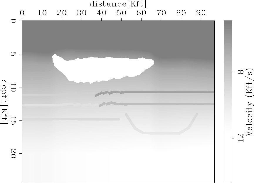
Figure 1 P-Wave Velocity Model

 

v_s
Figure 2 S-Wave Velocity Model

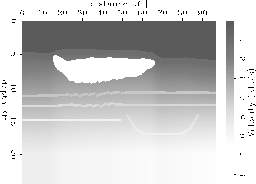Also shown is a synclinal structure (represents a paleochannel) below the two layers mentioned above, as well as a flat lens of sediment which starts on the left edge and stops abruptly underneath the salt. Both the syncline and lens are relatively low velocity layers. The S-wave velocity model seen in Figure 2 shows the same features, except that all the layers are consistently high velocity layers, and the layers in the faulted blocks remain at a constant velocity instead of abruptly changing as in the P-wave model.

 

ip_bar
Figure 3 P-Wave Impedance Model

 

is_bar
Figure 4 S-Wave Impedance Model

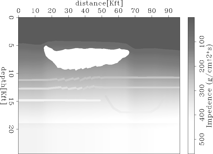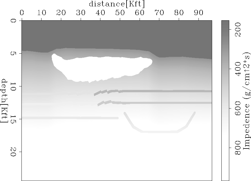
Impedances for the two models are shown in Figures 3 and 4. In the P-wave impedance model, large contrasts are seen for all of the features noted above, with the exception of the two slightly higher velocity layers seen at the left of the model, which end under the salt. In the S-wave impedance model, the impedance contrast remains constant for the two layers. A formula for reflectivity that is based on impedances is

$$R \; = \; \frac{Z_2-Z_1}{Z_1+Z_2} \;$$ (1)

where R is the reflectivity, and Z₁ and Z₂ are the impedances of the two layers.

From the formula, we can see that the magnitude of the reflection is independent of the position of the layers relative to each other. Rather, it is the sign which changes. So for high impedance over low, the reflection is in the same phase, while for low impedance over high, there is a 180⁰ phase shift Scheriff and Geldart (1995). For the purposes of imaging, the strength of the reflection becomes important, simply because stronger reflection coefficients mean that the layers will have higher amplitudes in the image. Referring back to Figures 3 and 4, we can see that P-wave energy should be strong from the top and bottom of the salt, as well as from all the other layers, with the exception of the two high velocity layers. However, these layers show a higher S-wave impedance contrast, and thus S-wave energy should be reflected relatively well.