


We assume that a set of data has been produced using active sources, that the time series response has been measured as a time series, and that these data have been Fourier transformed to produce the response matrix. At this point, there are two possibilities: (1) We could make direct use of the response matrix, or (2) we could continue processing the data by forming the time-reversal matrix and then computing the eigenvectors of the matrix. A third possibility that will be seen as a special case of the previous ones is that time-reversal data is collected and a single eigenvector is constructed by iteration on the physical system.
For our present purposes, in any of these cases we can take the diagonal entries of the response matrix as our data, or the diagonal entries of the rank one matrix formed from any eigenvector (computed or measured directly) of the time-reversal matrix as our data. We assume at first that there is a single target present. Then, for the eigenvectors, the diagonal entries will be real and positive numbers, but they will all contain a constant normalization factor associated with the norm of the eigenvector. For the response matrix, the diagonal entries will be complex and contain a constant factor associated with the scattering strength of the target. We eliminate the unit magnitude phase factor in response matrix diagonals by taking the magnitudes of these entries. Then, we see that in all the cases considered these diagonal data have (for homogeneous 3D media) the form
f_n = _i(4)^2 r_n-r_i^2
for n=1,...,N,
where ![]() is the magnitude of the scattering strength
for the response matrix data, or the norming constant for the
eigenvector data. The location of the target is
is the magnitude of the scattering strength
for the response matrix data, or the norming constant for the
eigenvector data. The location of the target is ![]() and the location of the nth element of the acoustic array
(having a total of N elements) is
and the location of the nth element of the acoustic array
(having a total of N elements) is ![]() .
.
Using these data, we want to construct a figure of merit that will identify the target location by producing either a noticeably high or a noticeably low value for any point in the imaging region to scanned. To accomplish this, we form the numbers
_n(r) = f_n(4)^2 r-r_n^2
where ![]() is the location of any point in the imaging region.
Then, we see that when
is the location of any point in the imaging region.
Then, we see that when ![]() is located at or very
near to the target, then
is located at or very
near to the target, then
_n(r_i) = _i
for all N functions ![]() . So we want to construct a figure of
merit that gives special significance to functions that are positive
and constant. But it is precisely this feature that distinguishes
the maximum-entropy approach to imaging. If we define an
entropy functional H such that
. So we want to construct a figure of
merit that gives special significance to functions that are positive
and constant. But it is precisely this feature that distinguishes
the maximum-entropy approach to imaging. If we define an
entropy functional H such that
H(p_1,...,p_N) = - k_n=1^N p_np_n,
with the constraint that the probabilities ![]() and
and ![]() , then we construct a maximum principle
based on the cost or objective functional
, then we construct a maximum principle
based on the cost or objective functional
J(p_1,...,p_N,) = H(p_1,...,p_N) + (p_n - 1),
where ![]() is the Lagrange multiplier for the constraint.
The maximum occurs when the constraint is satisfied, and when
is the Lagrange multiplier for the constraint.
The maximum occurs when the constraint is satisfied, and when
p_n = e^(-k)/k for all n=1,...,N. Thus, the maximum entropy occurs when all N states are equally probable.
 |

 |
We can turn this useful fact into an imaging principle by making a small modification in the foregoing derivation. If we define
p_n _n/c,
where ![]() , we see that the maximum-entropy functional
can be used as a means of identifying spatial locations at which the
various
, we see that the maximum-entropy functional
can be used as a means of identifying spatial locations at which the
various ![]() values converge to a constant. The constant k is
not important for this application and can be taken as unity.
The value of the Lagrange multiplier at the maximum can be determined
using (constant) and (pnconst) to be
values converge to a constant. The constant k is
not important for this application and can be taken as unity.
The value of the Lagrange multiplier at the maximum can be determined
using (constant) and (pnconst) to be
= 1 + (_i/c) = 1 - (N),
since ![]() at the target location.
Near the maximum of J, we can approximate it in either of two ways:
at the target location.
Near the maximum of J, we can approximate it in either of two ways:
J && - 1N_n(_n_i-1)^2 = 1 - 1N_n (_n_i)^2 or J && - 1N_n [(_n_i)]^2. For our present purposes, the second of these forms has proven to be somewhat preferable over the other. The normalizing constant N in this expression has no effect on the result, and whether we look for the minimum or maximum of our function is an arbitrary choice, so we can choose instead to study
J _n
[(_n_i)]^2.
which still requires that we know the scattering strength or norming
constant ![]() , which we may or may not know.
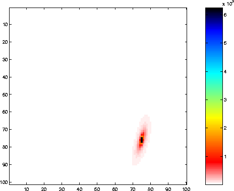
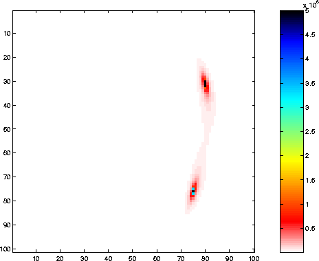
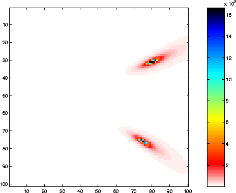
Figures 1 and 2 show the results obtained for one and two
targets using (Jtilde).
, which we may or may not know.
Figures 1 and 2 show the results obtained for one and two
targets using (Jtilde).
If we know ![]() , then we can image the target using
(Jtilde) directly. If we do not know
, then we can image the target using
(Jtilde) directly. If we do not know ![]() , then we need an estimate
of it. One convenient way of obtaining an estimate is by picking any one
of the
, then we need an estimate
of it. One convenient way of obtaining an estimate is by picking any one
of the ![]() values as the estimate. Clearly, this choice gives
a good approximation to the right
result at the target, but it will also cause some smearing of the
image. The imaging algorithm in this case is then based upon
values as the estimate. Clearly, this choice gives
a good approximation to the right
result at the target, but it will also cause some smearing of the
image. The imaging algorithm in this case is then based upon
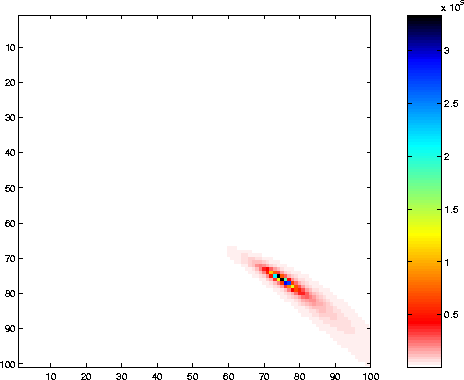
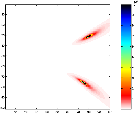
J_q _n
[(_n_q)]^2,
where q is any one of the values ![]() .This approach works and gives the results shown in Figures 3 and 4
(which should then be compared and contrasted with the results in Figures 1
and 2).
In these Figures, we chose q to be the transducer coordinate of the
one that measured the largest amplitude of all the transducers. We see
that the results are a little peculiar in the sense that the region of
disturbed values near the target location has a teardrop shape, and
the center of the teardrop also has some curvature directed away from
the center of the array. This
observation suggests that it might be preferable not to make any
particular choice of q, but instead to consider them all equally. We can do so
by symmetrizing the result as much as possible with data
available, and also possibly sharpen the image. This criterion results
in the imaging objective functional
.This approach works and gives the results shown in Figures 3 and 4
(which should then be compared and contrasted with the results in Figures 1
and 2).
In these Figures, we chose q to be the transducer coordinate of the
one that measured the largest amplitude of all the transducers. We see
that the results are a little peculiar in the sense that the region of
disturbed values near the target location has a teardrop shape, and
the center of the teardrop also has some curvature directed away from
the center of the array. This
observation suggests that it might be preferable not to make any
particular choice of q, but instead to consider them all equally. We can do so
by symmetrizing the result as much as possible with data
available, and also possibly sharpen the image. This criterion results
in the imaging objective functional
J _n,q [(_n_q)]^2 The result of using this criterion is shown in Figure 5, which should be compared directly to Figure 4.
 |
 |
 |
To understand a little better what this symmetrized maximum-entropy imaging scheme is doing to map the data into an image, we will expand (Jtilde2) so that
J &=&
_n,q [_n - _q]^2 &=& 2[_n,q (_n)^2 -
_n _n _q _q] &=& 2[N_n (_n)^2
- (_n _n)^2]
By defining an averaging operator over the functional values at the
locations of the N transducers such that ![]() , we see that (Jhat)
is of the form
, we see that (Jhat)
is of the form
J = 2N^2[<^2> -
<>^2]
and therefore shows that ![]() is a measure of the
fluctuations in
is a measure of the
fluctuations in ![]() at each location
in the region being mapped.
At the target location, the fluctuations vanish identically, since
they become equal to the constant
at each location
in the region being mapped.
At the target location, the fluctuations vanish identically, since
they become equal to the constant ![]() . Equation
(fluctuations) is very useful for two reasons: (1) it shows how
the modified maximum entropy imaging criterion is related to
fluctuations
in
. Equation
(fluctuations) is very useful for two reasons: (1) it shows how
the modified maximum entropy imaging criterion is related to
fluctuations
in ![]() , and (2) it points out that the form
, and (2) it points out that the form ![]() could have been postulated as our imaging criterion in the first
place, independent of the derivation provided here,
since it uses exactly the same features of the data to distinguish the
location of the target.
could have been postulated as our imaging criterion in the first
place, independent of the derivation provided here,
since it uses exactly the same features of the data to distinguish the
location of the target.