Examples

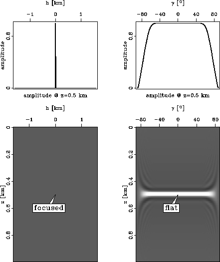
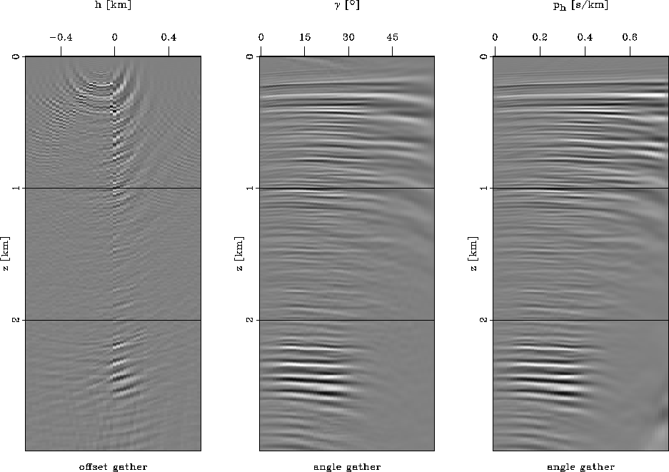
The first example represents a simple image-gather with one seismic event perfectly focused at zero offset (simplesyn). As expected, conversion to the angle-domain produces a flat event, which fattens out at high angles due to the finite sampling of the offset axis. This phenomenon is a consequence of the acquisition geometry, and not a property of the conversion to the angle-domain. The top panels of simplesyn show the amplitude of this simple event as a function of offset (left) and as a function of reflection angle (right). The conversion to angle produces a flat amplitude curve, as expected for this perfectly focused event. If this event is produced using true amplitude migration, then the reflectivity function of angle (AVA) produced by this algorithm is also true amplitude.

 

simplesyn
Figure 3 Ideal offset-domain and angle-domain common image gathers.

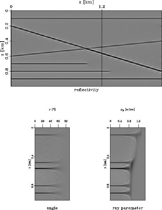
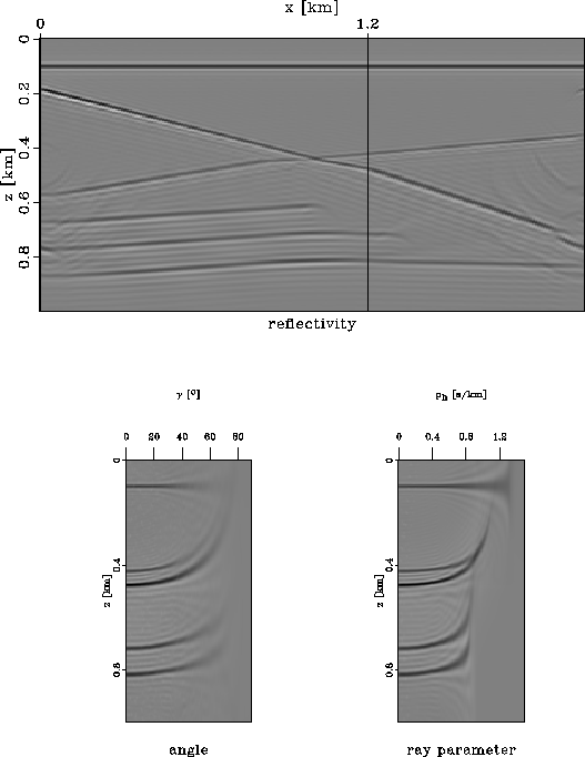
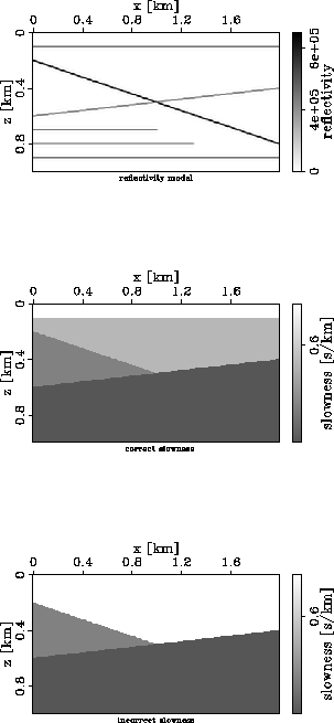
The second example is a 2D synthetic model with dipping reflectors at various angles. I generate the synthetic data using wavefield-continuation modeling and then image it using correct and incorrect velocities. The ADCIGs are flat for the case of correct velocity (frcimgC), but they are not flat for the case of incorrect velocity (frcimg0). The bottom panels show ADCIGs computed in the image and data spaces at the location indicated by the vertical line at 1.2 km. The velocity changes in the upper part of the model from 1.75 km/s in the correct model to 1.5 km/s in the incorrect one. Since I have simulated wide offset data, the deeper flat events do not suffer much from reduced angular coverage. However, the limited acquisition causes a reduction in angular coverage for the steeply dipping fault.

frcimgC and frcimg0 also show the different amplitude behavior between the image space and data space methods: for the image space method, the amplitudes decrease as a function of angle, while for the data space method, the amplitudes increase as a function of offset ray-parameter. This observation shows that AVA analysis on any of the two kinds of angle gathers is problematic (91).

 

frcmodel Figure 4 2D synthetic model: from top to bottom, reflectivity model, correct and incorrect slownesses.

 

frcimgC
Figure 5 Synthetic model imaged using the correct velocity model: section obtained by imaging at zero time and zero offset (top), angle gather created in the image space (bottom left), and angle gather created in the data space (bottom right).

 

frcimg0
Figure 6 Synthetic model imaged using the incorrect velocity model: section obtained by imaging at zero time and zero offset (top), angle gather created in the image space (bottom left), and angle gather created in the data space (bottom right).

The third example concerns a real dataset acquired over a region with fairly simple geology (kjamig). This dataset was first analyzed by (54) and it is part of the SEP data library. kjacig shows image gathers at x=7.5 km. As theoretically predicted, at the imaging step most of the energy is concentrated around zero offset. After the conversion to the angle-domain, almost all the events are flat, although some show slight moveout, indicating migration and/or velocity inaccuracies. For this example, too, we can observe the same difference in amplitude behavior of the data space versus the image space method as for the synthetic example in frcimgC and frcimg0.

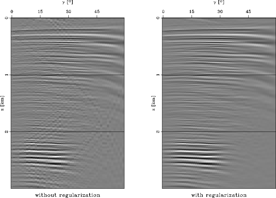
kjaeps demonstrates the effect of regularization in the angle-domain. In the left panel, I present an angle gather created without regularization ($\epsilon=0.0$), and on the right I present the same angle gather obtained with regularization ($\epsilon=1.0$), according to LSsol. The left panel is populated with artifacts caused by the non-uniform sampling of the ADCIG due to the radial trace transform in the Fourier domain. In contrast, the panel on the right shows fewer artifacts, which makes the reflections much easier to interpret.

 

kjamig
Figure 7 2D real data example: seismic section obtained by imaging at zero time and zero offset.

 

kjacig
Figure 8 2D real data example: from left to right, offset-gather (right panel) and angle gathers, computed in the image-space (middle panel) and the data-space (right panel)

 

kjaeps
Figure 9 2D real data example: a comparison of an angle gather obtained without regularization (left) and an angle gather obtained with regularization (right).

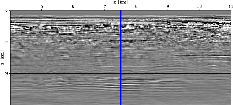
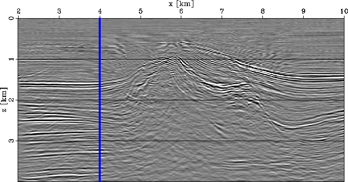
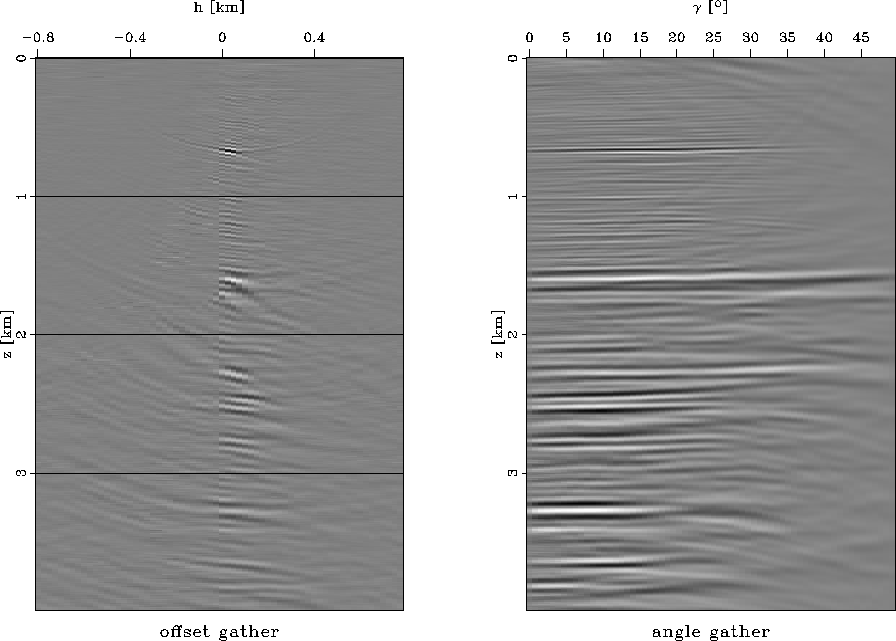
The fourth example concerns a 3D common-azimuth (9) data set from the North Sea (111). This dataset was donated to SEP by Elf and it is part of the SEP data library. l7dmig is an inline extracted from the 3D seismic cube and shows a salt body in the middle of the section, surrounded by fairly flat reflectors. l7dcig shows an image gather at x=4.0 km, presented in the offset-domain (left panel) and in the angle-domain (right panel). As before, most of the energy is imaged around zero offset, which translates in fairly flat events in the angle gather indicating that both the migration and the velocity model are correct. The geometry of the reflectors in this example are fairly simple, although the waves propagate through a complicated salt area.

 

l7dmig
Figure 10 3D common-azimuth example: seismic section obtained by imaging at zero time and zero offset. The vertical line corresponds to the CIGs in l7dcig.

 

l7dcig
Figure 11 3D common-azimuth example: offset-gather (left panel) and angle gather (right panel) corresponding to the vertical line in l7dmig.