Given data in the slowness,frequency domain ![]() I wish to
calculate the response in the time,offset domain P(t,x,y). This response
can be calculated by a double inverse slant stack and inverse fourier transform
of the input data.
I wish to
calculate the response in the time,offset domain P(t,x,y). This response
can be calculated by a double inverse slant stack and inverse fourier transform
of the input data.
In the discrete modeling scheme the integral over px and py is replaced by a discrete summation and the inverse fourier transform is replaced by an inverse discrete fourier transform.
There are problems with the slowness integration caused by
singularities in the modeling operation. Whenever the modeling
algorithm is performed for a slowness where pz is zero, or nearly
zero, for some wavetype there is a singularity or instability in the
modeling algorithm. These points occur when the waves are traveling
horizontally. The integration may be performed in a stable manner by
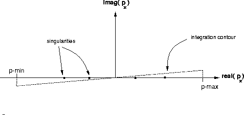
choosing to integrate in the complex slowness domain. I can choose
some other contour between pmin and pmax along which to
evaluate the integral. In my program I choose the contour lying along
the line between ![]() and
and ![]() .This contour is shown in figure
.This contour is shown in figure ![[*]](http://sepwww.stanford.edu/latex2html/cross_ref_motif.gif) . In practice I
choose
. In practice I
choose ![]() and I do not bother to sample the contour
along the small vertical parts of the contour.
and I do not bother to sample the contour
along the small vertical parts of the contour.
 |
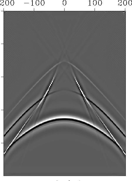
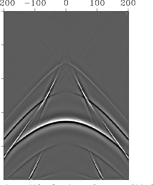
Figures ![[*]](http://sepwww.stanford.edu/latex2html/cross_ref_motif.gif) to
to ![[*]](http://sepwww.stanford.edu/latex2html/cross_ref_motif.gif) show the same data examples as before but now
they are calculated in the (x,t) domain. The most noticeable feature in the (x,t) domain is the triplication of the shear wave arrival. The amplitudes at
the cusps of the triplication are relatively high. This matches well with
theory and modeling results using other methods.
show the same data examples as before but now
they are calculated in the (x,t) domain. The most noticeable feature in the (x,t) domain is the triplication of the shear wave arrival. The amplitudes at
the cusps of the triplication are relatively high. This matches well with
theory and modeling results using other methods.
The P-wave direct arrival is clear in figure ![[*]](http://sepwww.stanford.edu/latex2html/cross_ref_motif.gif) but no direct shear
wave is seen because the integration in the slowness domain did not cover a
large enough range.
but no direct shear
wave is seen because the integration in the slowness domain did not cover a
large enough range.
 |
 |
 |
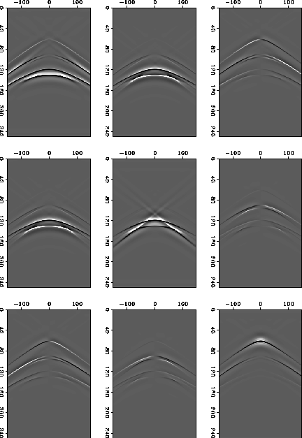
Figure ![[*]](http://sepwww.stanford.edu/latex2html/cross_ref_motif.gif) shows the results of modeling a full nine-component
shot gather. The shot is oriented at
shows the results of modeling a full nine-component
shot gather. The shot is oriented at ![]() to the symmetry axis of
an orthorhombic medium. There are clear shear wave conversions and
shear wave splitting in the data. The range of offsets and dips modeled was
not as great as the previous examples so the shear wave triplications are
not visible. The top row shows the x,y and z velocities for an x-traction.
The second rows shows the results for a y-traction and the third row for a
z-traction.
to the symmetry axis of
an orthorhombic medium. There are clear shear wave conversions and
shear wave splitting in the data. The range of offsets and dips modeled was
not as great as the previous examples so the shear wave triplications are
not visible. The top row shows the x,y and z velocities for an x-traction.
The second rows shows the results for a y-traction and the third row for a
z-traction.
 |