

Next: CONCLUSIONS
Up: APPLICATIONS
Previous: Well-log interpolation
Conventional velocity analysis is done in two steps. The first step is
to compute the semblances from CMP gathers. The second step is to
pick a velocity model that maximizes the semblances.
It is clear that if equation (1) is replaced by the Dix equation
|  |
(14) |
then the algorithm described earlier can be used for velocity analysis.
The constraint required in this problem is a smooth RMS velocity function.
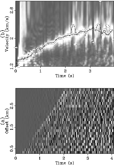
Figure ![[*]](http://sepwww.stanford.edu/latex2html/cross_ref_motif.gif) a shows a CMP gather from the Gulf of Mexico.
The semblance computed from this gather is displayed in Figure
a shows a CMP gather from the Gulf of Mexico.
The semblance computed from this gather is displayed in Figure ![[*]](http://sepwww.stanford.edu/latex2html/cross_ref_motif.gif) b.
I overlay the semblance with the picked velocity functions.
The stars indicates the picks when unconstrained optimization is used. These
picks form a rough and unrealistic velocity function. By using a weak
smoothness constraint, I get a velocity function plotted with the dashed curve.
Now the result becomes more acceptable. But still, the algorithm
picks the peak around 2.3 second, that is known to be caused by a dipping bed.
I further increase the smoothness constraint and obtain the final picks
plotted with a solid curve in Figure
b.
I overlay the semblance with the picked velocity functions.
The stars indicates the picks when unconstrained optimization is used. These
picks form a rough and unrealistic velocity function. By using a weak
smoothness constraint, I get a velocity function plotted with the dashed curve.
Now the result becomes more acceptable. But still, the algorithm
picks the peak around 2.3 second, that is known to be caused by a dipping bed.
I further increase the smoothness constraint and obtain the final picks
plotted with a solid curve in Figure ![[*]](http://sepwww.stanford.edu/latex2html/cross_ref_motif.gif) b. This result is
reasonably good.
halevel
b. This result is
reasonably good.
halevel
Figure 7 Velocity picking: (a) a common midpoint gather; (b) semblance overlain with
the results of velocity picking. The stars show the locations of the maximum
of semblance for each time samples. The dashed curve shows the velocity picking
with a weak constraint. The final result is shown by the solid curve.


Next: CONCLUSIONS
Up: APPLICATIONS
Previous: Well-log interpolation
Stanford Exploration Project
12/18/1997
![[*]](http://sepwww.stanford.edu/latex2html/cross_ref_motif.gif) a shows a CMP gather from the Gulf of Mexico.
The semblance computed from this gather is displayed in Figure
a shows a CMP gather from the Gulf of Mexico.
The semblance computed from this gather is displayed in Figure ![[*]](http://sepwww.stanford.edu/latex2html/cross_ref_motif.gif) b.
I overlay the semblance with the picked velocity functions.
The stars indicates the picks when unconstrained optimization is used. These
picks form a rough and unrealistic velocity function. By using a weak
smoothness constraint, I get a velocity function plotted with the dashed curve.
Now the result becomes more acceptable. But still, the algorithm
picks the peak around 2.3 second, that is known to be caused by a dipping bed.
I further increase the smoothness constraint and obtain the final picks
plotted with a solid curve in Figure
b.
I overlay the semblance with the picked velocity functions.
The stars indicates the picks when unconstrained optimization is used. These
picks form a rough and unrealistic velocity function. By using a weak
smoothness constraint, I get a velocity function plotted with the dashed curve.
Now the result becomes more acceptable. But still, the algorithm
picks the peak around 2.3 second, that is known to be caused by a dipping bed.
I further increase the smoothness constraint and obtain the final picks
plotted with a solid curve in Figure ![[*]](http://sepwww.stanford.edu/latex2html/cross_ref_motif.gif) b. This result is
reasonably good.
b. This result is
reasonably good.
