

Next: Conclusions
Up: Karrenbach: 3d time slice
Previous: Integral formulation
In order to sum along the diffraction surface of a scattering point,
the energy
can be summed along circles in the time-slice representation of a 3D data
volume. This process can be approximated by multiplying the
2D Fourier transform
of each time slice by a cosine filter, corresponding to the
radius of the
intersection of the time slice with the diffraction surface.
The spatial Fourier domain
is computationally attractive, since convolution in space reduces to a simple
multiplication in the spatial frequency domain.
The first task is then to perform a 2D Fourier transform of all the
time slices. For that I used the CMSSL library on the Connection Machine,
which includes an optimized multidimensional FFT subroutine.
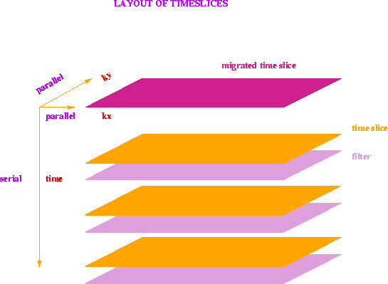
Figure ![[*]](http://sepwww.stanford.edu/latex2html/cross_ref_motif.gif) shows the layout of the transformed time slices and their filters.
The 3D data cube has now one serial (temporal) dimension and two parallel axes,
namely kx and ky (spatial frequencies).
Each spatial
frequency in a time slice is handled by a separate processor,
and all the spatial frequencies
are calculated independently from each other.
For each spatial frequency component the values for all times and three filter
coefficients are stored in local memory.
No interprocessor communication is necessary to migrate each frequency
component. All filtered time-slice components that are summed,
come directly from each processor's local memory.
Thus the spatial frequency domain maps perfectly onto the Connection Machine
layout.
The summation over the diffraction surface proceedes along the
serial time axis,
an is carried out for all spatial frequency components simultaneously.
shows the layout of the transformed time slices and their filters.
The 3D data cube has now one serial (temporal) dimension and two parallel axes,
namely kx and ky (spatial frequencies).
Each spatial
frequency in a time slice is handled by a separate processor,
and all the spatial frequencies
are calculated independently from each other.
For each spatial frequency component the values for all times and three filter
coefficients are stored in local memory.
No interprocessor communication is necessary to migrate each frequency
component. All filtered time-slice components that are summed,
come directly from each processor's local memory.
Thus the spatial frequency domain maps perfectly onto the Connection Machine
layout.
The summation over the diffraction surface proceedes along the
serial time axis,
an is carried out for all spatial frequency components simultaneously.
cmlayout
Figure 1 The spatial frequencies of individual time slices and filters are laid out on the Connection Machine in parallel. The time axis is kept as a serial dimension. No interprocessor communication is necessary to filter and sum individual spatial frequency components.
 filter
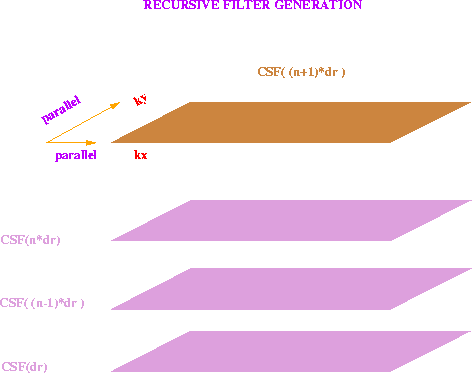
Figure 2 Time-slice filters CSF( (n+1)*dr ) are generated by recursion as needed. This can be done for each spatial frequency independently. No interprocessor communication is necessary.

The pseudocode for migrating time slices is

- 2D FFT of all time slices to be summed

- For each increment in diffraction radius
-

-
- Generate time-slice filter CSF
-
- Interpolate time slice
-
- Filter time slice
-
- Sum into migrated slice
-


- Inverse 2D FFT of migrated time slices
The most efficient way to obtain the
filter values for each slice that is summed, is to apply the
trigonometric recursion
|  |
(3) |
where the subscript is a multiplication factor in the argument of CSF, such
that  , with the initialization
CSF0=1 and
  .Thus each processor can calculate the new filter coefficient
for each slice which is summed, with just three-floating point operations.
Starting the summation at the vertex of the diffraction surface is advantageous
in that the migration aperture does not have to be fixed at the
beginning of the process. One can use this for an interactive session where
the migration aperture can be chosen by inspection.
The algorithm, as implemented now, is running typically at a speed of
190 Mflops on a 4k processor machine. It seems to me fast enough to be
used as a tool for a very simple interactive 3D migration velocity analysis.


Next: Conclusions
Up: Karrenbach: 3d time slice
Previous: Integral formulation
Stanford Exploration Project
12/18/1997
![[*]](http://sepwww.stanford.edu/latex2html/cross_ref_motif.gif) shows the layout of the transformed time slices and their filters.
The 3D data cube has now one serial (temporal) dimension and two parallel axes,
namely kx and ky (spatial frequencies).
Each spatial
frequency in a time slice is handled by a separate processor,
and all the spatial frequencies
are calculated independently from each other.
For each spatial frequency component the values for all times and three filter
coefficients are stored in local memory.
No interprocessor communication is necessary to migrate each frequency
component. All filtered time-slice components that are summed,
come directly from each processor's local memory.
Thus the spatial frequency domain maps perfectly onto the Connection Machine
layout.
The summation over the diffraction surface proceedes along the
serial time axis,
an is carried out for all spatial frequency components simultaneously.
shows the layout of the transformed time slices and their filters.
The 3D data cube has now one serial (temporal) dimension and two parallel axes,
namely kx and ky (spatial frequencies).
Each spatial
frequency in a time slice is handled by a separate processor,
and all the spatial frequencies
are calculated independently from each other.
For each spatial frequency component the values for all times and three filter
coefficients are stored in local memory.
No interprocessor communication is necessary to migrate each frequency
component. All filtered time-slice components that are summed,
come directly from each processor's local memory.
Thus the spatial frequency domain maps perfectly onto the Connection Machine
layout.
The summation over the diffraction surface proceedes along the
serial time axis,
an is carried out for all spatial frequency components simultaneously.

