Next: CONCLUSIONS
Up: Mo and Bai: Boundary
Previous: Absorbing boundary conditions for
We develop absorbing boundary conditions for Zhiming Li's (1986) migration
equation.
In the space-time domain, the transforms are:
|  |
(14) |
and the inverse transforms are:
|  |
(15) |
In the frequency-wavenumber domain, the transforms are
|  |
(16) |
Then the original dispersion relation changes to
|  |
(17) |
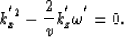
Because in coordinate transformation rotation, the kx axis is fixed,
so the transformation is actually a rotation with kx
as the symmetry axis.
After coordinate rotation, the conic surface for kx'>0 is the same
as the conic surface for kx>0, similarly for kx'<0
versus kx<0. So coordinate transformation does not change the
propagation directions of the leftward and rightward traveling waves.
We apply the leftgoing (or rightgoing) wave equation in the new coordinate
system as a boundary condition, then we obtain the absorbing
boundary conditions:
|  |
(18) |
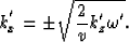
To get the difference equation in the space-time domain, we must
approximate the square root in (18). The order of kz' in the
approximate equation must be no more than one, for only upcoming
waves are to be present in our migration wavefield.
Because under coordinate transformation only our viewing angle is changed,
the object (cone) itself is not changed. We can use the
approximate formulas in the last section. After coordinate rotation, A1 and
A2 change into:
|  |
(19) |
and
|  |
(20) |
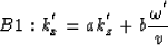
In the space-time domain, B1 and B2 correspond to:
| 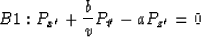 |
(21) |
and
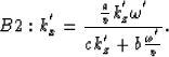
| 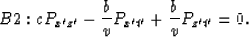 |
(22) |
Because of coordinate transformation, the (x-z) plane changes to
the (x'-z')
plane, then the rightgoing wave must be considered in
thethe new (x'-z') plane.
In the (x,z,t) domain, the rightgoing wave is
|  |
(23) |
where  , and
, and  .
PI could not be a downgoing wave, for in our migration wavefield there
is only an upcoming wave component, no downgoing wave.
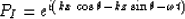
After coordinate transformation,
.
PI could not be a downgoing wave, for in our migration wavefield there
is only an upcoming wave component, no downgoing wave.
After coordinate transformation,
| ![\begin{displaymath}
P_{I}^{'}=e^{i[kx^{'}\cos\theta+{k \over \sqrt{2}}z^{'}(1-\sin\theta)
-{\omega \over \sqrt{2}}t^{'}(1+\sin\theta)]}.\end{displaymath}](img29.gif) |
(24) |
Let the right boundary reflection coefficient be R, then the wavefield
near the boundary is:
![\begin{displaymath}
P(x^{'},z^{'},t^{'})=P_{I}^{'}+ P_{R}^{'}
=e^{i[kx^{'}\cos...
...'}(1-\sin\theta)
-{\omega \over \sqrt{2}}t^{'}(1+\sin\theta)]}\end{displaymath}](img30.gif)
| ![\begin{displaymath}
+e^{i[-kx^{'}\cos\theta+{k \over \sqrt{2}}z^{'}(1-\sin\theta)
-{\omega \over \sqrt{2}}t^{'}(1+\sin\theta)]}.\end{displaymath}](img31.gif) |
(25) |
Substituting the above equation into boundary equations, we get:
|  |
(26) |
and
|  |
(27) |
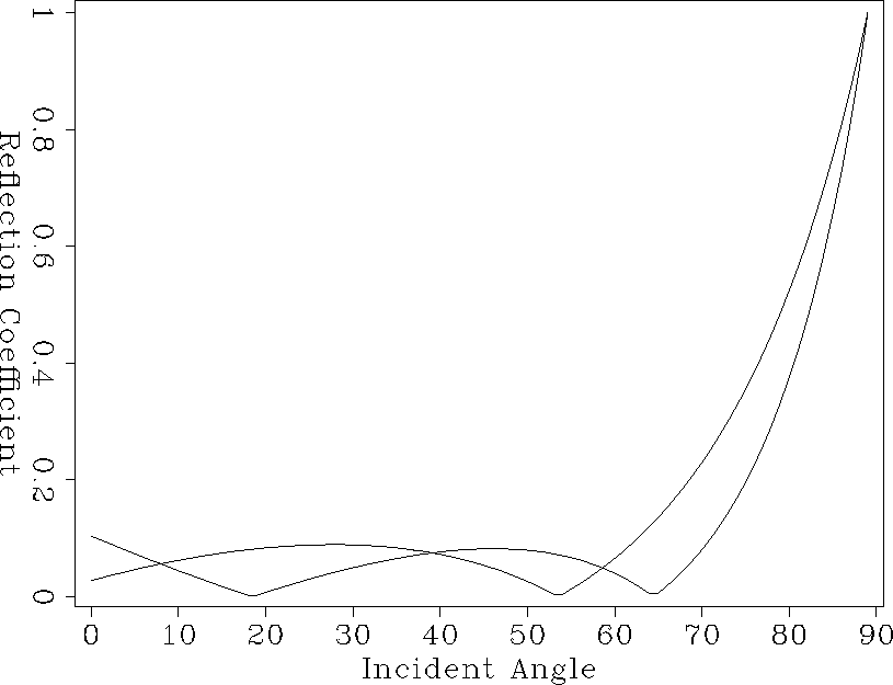
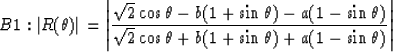
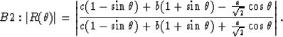
For a reflection coefficient R0=0.1,we find the coefficients
a, b, and c, by trial and error, so that
 in over as large a
  range as possible.
B1: a=1, b=0.35
B2: a=17, b=2, c=13.
In Figure 3, the reflection coefficients for B1, B2 are plotted.
We apply the condition B2 to migrate three different frequency
wavelets, and the results are displayed in Figure 4.
fig3
Figure 3
Graph of reflection coefficients for boundary conditions
B1 and B2.


Figure 4:
Migration of three different frequency wavelets,(left) zero-value
boundary, (right) absorbing boundary condition B2.
|
Next: CONCLUSIONS
Up: Mo and Bai: Boundary
Previous: Absorbing boundary conditions for
Stanford Exploration Project
12/18/1997