


When the problem is linear we should obtain
the model that ``best'' fit the data in only one iteration. When
the problem is non-linear one approach is to solve it as a sequence
of linearized steps. We usually call these steps external
iterations, to differentiate them from the internal iterations
needed to solve each linear problem
when using iterative techniques such as conjugate gradients. Ideally, if the
problem has n unknowns, each external iteration should
consists of m CG-steps (m internal iterations), where ![]() is the number of different singular values. When dealing with field
data, however, we might not be able to do this
because of the
presence of the noise. Noise can affect the solution of
each linearized problem in the following ways: (a)
It might be amplified in the model by the smallest singular values
recovered
when m iterations are performed, (b) It might affect considerably
the accuracy of the search directions and consequently, the position
of the minimum
associated with the solution. Therefore,
we have to deal carefully with the noise.
is the number of different singular values. When dealing with field
data, however, we might not be able to do this
because of the
presence of the noise. Noise can affect the solution of
each linearized problem in the following ways: (a)
It might be amplified in the model by the smallest singular values
recovered
when m iterations are performed, (b) It might affect considerably
the accuracy of the search directions and consequently, the position
of the minimum
associated with the solution. Therefore,
we have to deal carefully with the noise.
 |

 |
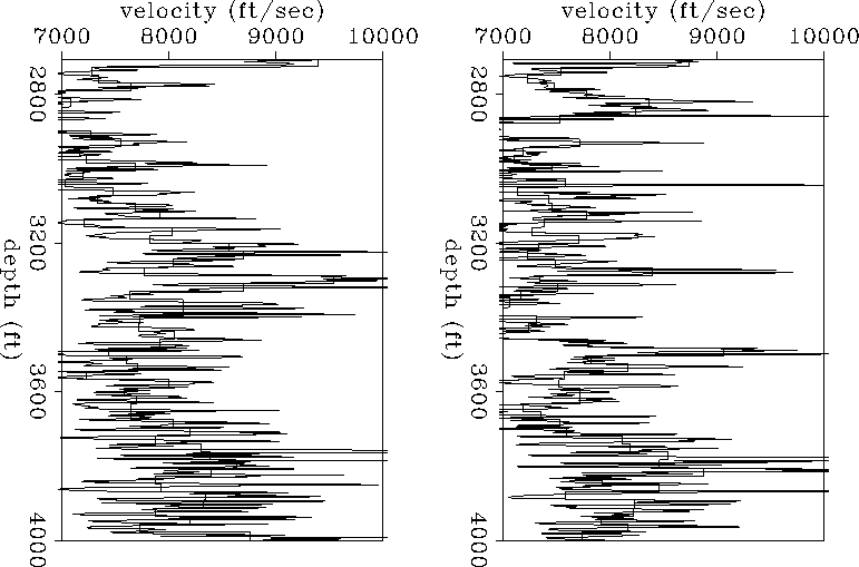
Under the straight-ray assumption,
only one external iteration was needed in the 1-D inversion to find
the model shown in Figure ![[*]](http://sepwww.stanford.edu/latex2html/cross_ref_motif.gif) .
By selecting the layer
thickness appropriately, we were able to perform the
CG-iterations required to reach convergency without being
much affected by the noise:
thicker layers
damped the solution
whereas thiner layers introduced instabilities.
In 2-D, however, the situation is different.
In this case we found that the results were
more sensitive to noise in the data than 1-D results. This is not
surprising because now we are trying to estimate
horizontal variations in Sz which, as explained before,
are related to the smallest
singular values of the problem (that amplify the noise).
.
By selecting the layer
thickness appropriately, we were able to perform the
CG-iterations required to reach convergency without being
much affected by the noise:
thicker layers
damped the solution
whereas thiner layers introduced instabilities.
In 2-D, however, the situation is different.
In this case we found that the results were
more sensitive to noise in the data than 1-D results. This is not
surprising because now we are trying to estimate
horizontal variations in Sz which, as explained before,
are related to the smallest
singular values of the problem (that amplify the noise).
Because of the sensitiveness to the noise of the 2-D inversion, it is
necessary
to avoid ``many'' CG-iterations at each linearized
step.
After several tests combining in different ways external and internal
iterations with mean-average
smoothing of the slowness model, we adopted a conservative
approach to minimize the error (12). The approach consisted of the following
steps:
(1) Compute traveltimes in the given model, calculate the matrix ![]() and
find the residuals. (2) Approximate the solution of the linear
problem (11)
by applying few (typically one or two) CG-iterations. (3) Smooth the
updated slowness
model. (4) Repeat all the previous steps until there is no reduction in the
sum (12). When this happens,
either quit or increase the number of CG-iterations by one and check
if further reductions in the mismatch are obtained.
If the problem
is linear, the solution is not obtained in only one iteration
because of the presence of the noise.
and
find the residuals. (2) Approximate the solution of the linear
problem (11)
by applying few (typically one or two) CG-iterations. (3) Smooth the
updated slowness
model. (4) Repeat all the previous steps until there is no reduction in the
sum (12). When this happens,
either quit or increase the number of CG-iterations by one and check
if further reductions in the mismatch are obtained.
If the problem
is linear, the solution is not obtained in only one iteration
because of the presence of the noise.
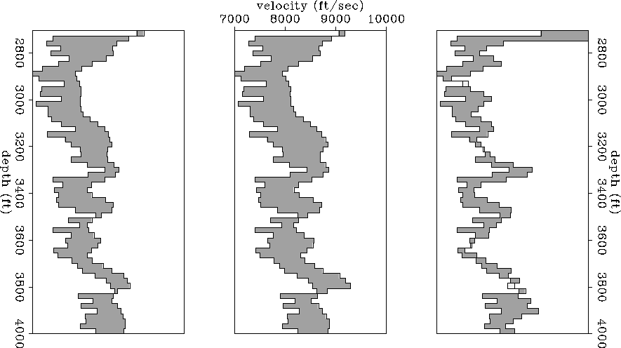
When the previous procedure was applied to estimate
an isotropic model from the data, we obtained the image
shown in Figure (error = 0.54 ms). In this case,
the unknown model was discretized into
131 x 26 square cells (10 ft2 each). It is interesting
to notice that adding more degrees of freedom
in structure (more cells) does not improve substantially the parameter error
obtained with 28 times less degrees of freedom in the 1-D anisotropic inversion.
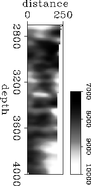
The model shown in Figure is similar to the
one obtained by Harris et al. (1990b).
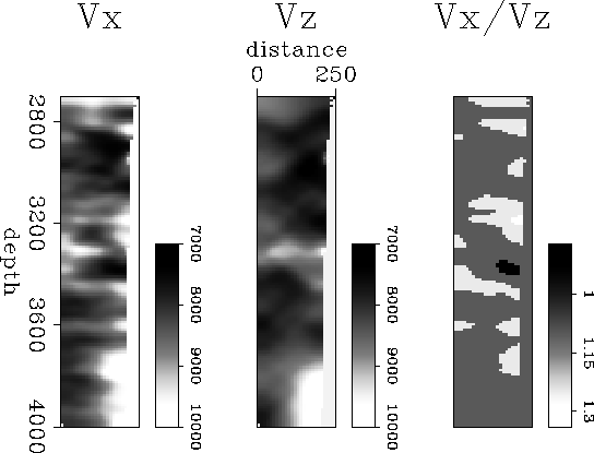
The result of the
anisotropic inversion is shown in Figure (error =
0.45 ms). Notice
that Vx is remarkably similar to Viso, like in the 1-D inversion.
The
main difference between these two images is that in
Vx (Figure )
the events tend to be
more horizontally smeared that in Viso (Figure ).
This was expected from the synthetic example shown in Figure .
The events in the vertical component of the velocity tend to be smeared in the direction of the steepest rays and the spatial resolution in this component is poor when compared with Viso and Vx. This is because Vz is not properly sampled by the recording geometry. In the 1-D case, as we said before, this lack of information is compensated by assuming a layered model, which allows to perform more CG-iterations without having problems with the noise. In 2-D this is not possible and therefore, the results obtained can be in a stage where Vx is close to convergency but Vz is far from that point. This in turn introduces artificial anisotropy.
Because Vx and Vz cannot be estimated at the same resolution (at least using only this type of recording geometry), it is not possible to estimate spatial variations in
 |
velocity anisotropy
(the ratio Vx / Vz for example) at the
same scale of the variations in velocity. Still, an image that shows
variations in velocity anisotropy can be useful if it accounts only
for the large scale variations that are well resolved by the inversion.
Such an image is shown in Figure . This image
is divided into four areas: highly anisotropic, moderately anisotropic,
isotropic and anisotropic with Vz > Vx.
We can see that most of the model is isotropic whereas the anisotropic areas
are associated with high isotropic-velocity zones, possibly shales.
The mismatch estimated by equation (12) (error)
decreases roughly 50![]() from the homogeneous to the
1-D inversion and about 60
from the homogeneous to the
1-D inversion and about 60![]() from the homogeneous to the
2-D inversion. This means that for this data set, by trying to estimate
lateral variations in the medium
(small singular values)
only a 10
from the homogeneous to the
2-D inversion. This means that for this data set, by trying to estimate
lateral variations in the medium
(small singular values)
only a 10![]() reduction in the mismatch is gained
with respect to
estimating only vertical variations in the model
(largest singular values).
reduction in the mismatch is gained
with respect to
estimating only vertical variations in the model
(largest singular values).
 |