Next: Conclusions
Up: Nichols: Wavefield separation
Previous: Calculation of the P-S
I modeled the response of a simple one layered model to a unit
displacement source on the free surface. The surface layer is the
orthorhombic medium used in my earlier examples. The modeling
algorithm is the phase shift scheme I described in an earlier report
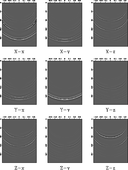
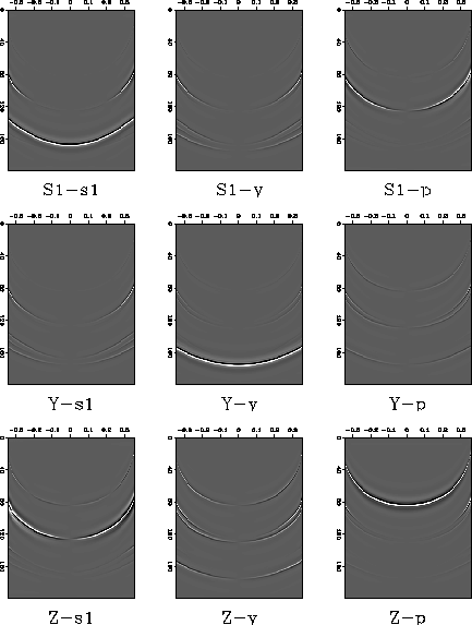
(Nichols, 1991). A synthetic nine-component gather is shown in
Figure ![[*]](http://sepwww.stanford.edu/latex2html/cross_ref_motif.gif) . It is displayed in the
. It is displayed in the  domain. The X-x section
clearly has many different wavetypes present in the gather. The first
event is the P-p wave the second is the P-s and S-p arrivals. The last
two events are the two S-s wave arrivals. The two shear waves are
split even at zero slowness because this is an orthorhombic medium.
domain. The X-x section
clearly has many different wavetypes present in the gather. The first
event is the P-p wave the second is the P-s and S-p arrivals. The last
two events are the two S-s wave arrivals. The two shear waves are
split even at zero slowness because this is an orthorhombic medium.
orig
Figure 4 Synthetic nine-component shot gather
shown in the domain. Many different wavetypes can
be seen on each component.


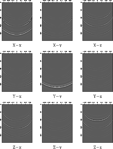
Source and receiver rotation by  gives the gather shown in
Figure . The horizontal component sections have been
diagonalized at zero slowness where the rotation is the exact operator
for S-wave separation. The two shear waves have been reasonably
separated at all but the highest slownesses. However the horizontal
component sections in the rotated reference frame still contain P-p
energy and converted wave energy.
gives the gather shown in
Figure . The horizontal component sections have been
diagonalized at zero slowness where the rotation is the exact operator
for S-wave separation. The two shear waves have been reasonably
separated at all but the highest slownesses. However the horizontal
component sections in the rotated reference frame still contain P-p
energy and converted wave energy.
rotated
Figure 5 Nine component gather after source and receiver rotation by . The two shear wavetypes have been totally separated at zero slowness and approximately separated at other slownesses.
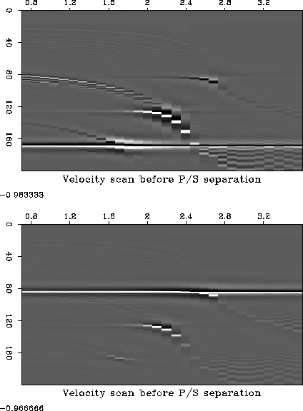
Figure shows the constant velocity stack panels for the
X-x and Z-z components of the data. There is coherent energy at three
separate places on the panel. These correspond to the different
reflection events, P-P, P-s/S-p and S-s.
vel-rot
Figure 6 Constant velocity stack panels for
the rotated data. The top panel is the X-x component and the bottom
panel is the Z-z component.
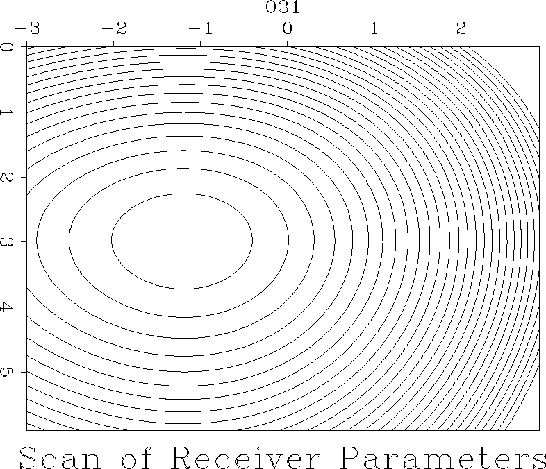
The next stage of the separation process is to estimate the P/S1
separation coefficients for the receiver operator.
Figure is a contour plot of the ``F2'' objective
function for a range of separation coefficients. The values of the
coefficients at the minimum of this plot were used in a receiver
separation operator that was applied to the synthetic data. The
resulting gather is displayed in Figure . The first
column of this plot should now correspond to an ``S1'' receiver.
Therefore there should be no upcoming P-waves visible on the first
column. Similarly the last column should now correspond to a
``P-receiver'' there are no upcoming S-waves visible in this column.
S-p waves are still visible in the bottom right section because the Z
source generates both P- and S-waves. Figure shows
the constant velocity stacks after receiver separation. There is
almost no energy at the S-s wave velocity on the Z-p velocity panel
and no energy at the P-p wave velocity on the X-s1 velocity panel.
rec-obj
Figure 7 Contour plot of the F2 objective function
for the receiver separation parameters.
|
|  |
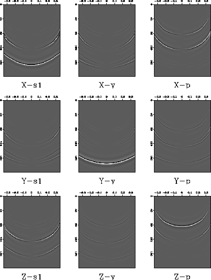
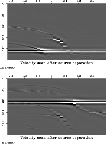
A similar P/S1 separation operator was estimated for the source
operator and applied to the data. The result is shown in
Figure . Although the separation is not complete at the
highest slownesses the P- and S1-waves have been completely
separated for a wide range of slownesses around zero slowness. In
particular the separation of the two converted wavetypes has been
particularly successful, compare the original data in
Figure with the final separation result in
Figure . The regions where the separation is
unsuccessful correspond the to regions in which the first order
approximation breaks down. In this example I have not yet applied the
final stage of the process, the P/S2 wave separation.
rec-sep
Figure 8 Nine-component gather after
application of the receiver P/S1 operator. The upcoming P waves have been
removed from the first column and the upcoming S1-waves have been
removed from the third column.
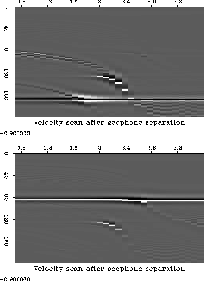
vel-recsep
Figure 9 Constant velocity stack panels
for the data after receiver P/S1 separation. The top panel is the
X-s1 component and the bottom panel is the Z-p component. There is
little upcoming P-wave energy on the X-s panel and little
upcoming S1-wave energy on the Z-p panel.
src-sep
Figure 10 Nine component gather after
application of the source and receiver P/S1 operators. The downgoing P
waves have been removed from the first row and the downgoing S1-waves
have been removed from the third row.
vel-srcsep
Figure 11 Constant velocity stack panels
for the data after source and receiver P/S1 separation. The top panel
is the S1-s1 component and the bottom panel is the P-p component. The
separation is not complete but most of the unwanted energy has been
removed.
Next: Conclusions
Up: Nichols: Wavefield separation
Previous: Calculation of the P-S
Stanford Exploration Project
12/18/1997