Next: INTERPOLATION
Up: Ji: Trace Interpolation
Previous: Ji: Trace Interpolation
The phrase ``spectral estimation'' has been used for a long time to
represent correct estimation of the power spectrum of a time series.
Here, I use the phrase to mean estimation of the spectrum which is
supposed to result from interpolation.
Let us consider a plane wave, which is a linear event in the time-space
(t-x) domain, and its spectrum, which is also a linear event in
the frequency-wavenumber (f-k) domain.
If we sample densely enough to avoid aliasing in the time direction and
sparsely along the space direction, the spectrum of the plane wave will
show spatial aliasing as is then the case in a conventional seismic survey.
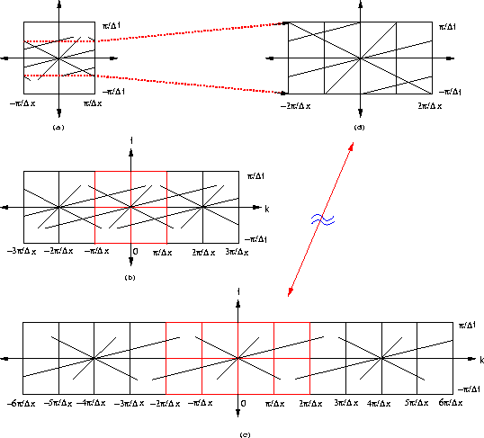
Figure 1a shows a spectrum containing several linear events with
spatial aliasing.
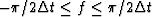
Figure 1b shows the spectrum of such data from
 to
to  along the wavenumber axis.
From Figure 1b, we can see that the aliasing is caused by a portion of
the original spectrum shifted by
along the wavenumber axis.
From Figure 1b, we can see that the aliasing is caused by a portion of
the original spectrum shifted by  , which is still located
in the region
, which is still located
in the region  to
to  along the wavenumber axis.
If we oversample with
along the wavenumber axis.
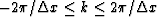
If we oversample with  =
=  ,the spectrum which caused the aliasing effect will be shifted
further, to
,the spectrum which caused the aliasing effect will be shifted
further, to  (Figure 1c).
As a result, one of the aliased events will disappear where
(Figure 1c).
As a result, one of the aliased events will disappear where
 .On the other hand, we can mimic a spectrum like Figure 1c by
taking the aliased spectrum only from
.On the other hand, we can mimic a spectrum like Figure 1c by
taking the aliased spectrum only from
 , as in Figure 1d.
fig1
Figure 1 (a) The spatially aliased spectrum. (b) The spatially aliased spectrum with replication. (c) The oversampled spectrum which is the spectrum after interpolation. (d) The spectrum estimated from the aliased spectrum.

Let us describe a linear event in the spectrum as a line segment
where a = df/dk is the inverse dip of a linear event, and f and k are
defined on 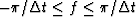 and
and
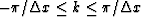 , respectively.
Then, the aliased event can be described by a shifted line:
, respectively.
Then, the aliased event can be described by a shifted line:
| 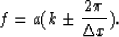 |
(2) |
If we oversampled by 1/N times the given sampling interval
in the space domain, the line will be
| 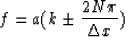 |
(3) |
where k is defined on  .By pulling out N from the bracket on the right-hand side of equation (3)
and changing variables according to f'=f/N and k'=k/N,
we find that equation (3) becomes
.By pulling out N from the bracket on the right-hand side of equation (3)
and changing variables according to f'=f/N and k'=k/N,
we find that equation (3) becomes
| 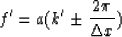 |
(4) |
where f' and k' are defined on
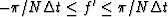 and
and
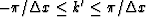 , respectively.
Equation (4) tells us that, by taking a portion of the given spectrum,
we can obtain a spectrum which corresponds to the spectrum after
interpolation.
, respectively.
Equation (4) tells us that, by taking a portion of the given spectrum,
we can obtain a spectrum which corresponds to the spectrum after
interpolation.
Next: INTERPOLATION
Up: Ji: Trace Interpolation
Previous: Ji: Trace Interpolation
Stanford Exploration Project
12/18/1997