EXAMPLES

For the sake of simplicity, I demonstrate the method by interpolating one dimensional time sequences. The data sequence shown in the following examples is a segment of a trace from a field dataset. The original trace has a uniform time sampling interval of 2 ms and a maximum frequency of 160 Hz. To prevent the signal from aliasing after random sub-sampling, the signal is low-passed to 100 Hz. Figure shows two examples of interpolating the randomly sub-sampled signal. Both examples have 32% randomly missing samples, but the distributions of the missing samples are different. The distribution of the missing samples in the first example is close to uniform, while the missing samples in the second example are clustered into a few groups. From Figure , we see that the results of the interpolation are satisfactory. Figure compares the amplitude spectra computed from the original signal and from the signal with random missing samples, respectively. The results indicate that the algorithm can accurately estimate the spectrum of an irregularly sampled signal.

 

interp
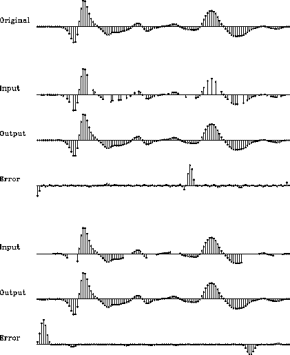
Figure 2 Two examples of interpolating irregularly sampled data. The top trace shows a segment of seismic data. The three traces in the middle show data before and after interpolation, and interpolation error, which is magnified by a factor of 500. The three traces at the bottom show another example in which the missing samples are clustered. The error in this second example is magnified by a factor of 40.

 

specirre Figure 3 Amplitude spectra: The solid curve is computed from the original signal; The dashed curve is computed from the signal with random missing samples.