


When solving the inverse problem, the goal is to estimate two different sets of coupled unknowns: the model parameters and the ray paths. The usual way to decouple them is by invoking Fermat's principle, which ``justifies'' the trick of assuming one to estimate the other in an iterative fashion, as long as the magnitude of the changes from one step to the next are kept small.
Once the ray paths have been estimated, the system of nonlinear
equations (5) needs to be solved in order to find a new model
where rays are going to be traced again.
One way to do this is as a sequence
of linearized steps starting from a given initial model
![]() . The first step is to approximate
(5) by its first order Taylor
series expansion centered about a given model
. The first step is to approximate
(5) by its first order Taylor
series expansion centered about a given model ![]() :
:
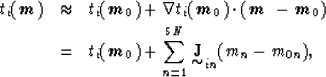 |
||
| (7) |
![]()
If we assume that ![]() represents one component of the
vector
represents one component of the
vector ![]() of measured traveltimes,
we can compute the perturbations
of measured traveltimes,
we can compute the perturbations
![]() once
the traveltimes in the reference model
once
the traveltimes in the reference model ![]() has been calculated.
The perturbation
has been calculated.
The perturbation ![]() is the solution of the following
system of equations
is the solution of the following
system of equations
| (8) |
In practice, only a fraction r of the correction
![]() is added to the given model
is added to the given model
![]()
The system of linear equations (8) will be solved using the LSQR variant of the conjugate gradients algorithm (Nolet, 1987)