Next: Migrations
Up: A MARINE DATA EXAMPLE
Previous: Marine data and preprocessing
Next I ran the Monte Carlo automatic velocity fitting algorithm on all 300
velocity semblance scans. The total CPU time requires an average of
10 CPU seconds per velocity scan on an IBM RS/6000 Model 530 with the following
search parameters. For the initial parametric interval velocity estimate,
I searched over the surface velocity range vo = 1.4-1.6 km/s in 0.5 km/s
increments, the velocity gradient parameter range  = 0.1-0.5 km/s/s
in 0.1 km/s/s increments, and the time exponent range
= 0.1-0.5 km/s/s
in 0.1 km/s/s increments, and the time exponent range  = 0.1-1.0 in
0.1 unit increments.
= 0.1-1.0 in
0.1 unit increments.
For the subsequent Monte Carlo search, I used the
following parameters: 20 interval velocity layers per second, a maximum
adjacent vertical velocity increment of 0.2 km/s, a random walk velocity
search corridor bound of 0.8 and 1.2 times the best current interval velocity
model, a surface velocity of 1.525 km/s constant from 0.0-0.2 seconds,
a global minimum and maximum interval velocity of 1.525 and 3.0 km/s,
a standard deviation of 10% of the best current vi value for the
random velocity perturbations drawn from a uniform distribution, a
convergence error tolerance of 0.1% of the peak maximum semblance integral
value, a ``stale'' convergence criterion of 10 unchanged consecutive
random walks, and a maximum of 100 random walks each consisting of 100
random steps, resulting in a maximum of 10,000 random trial interval
velocity models. These parameters were discussed in the previous section
explaining the Monte Carlo method.
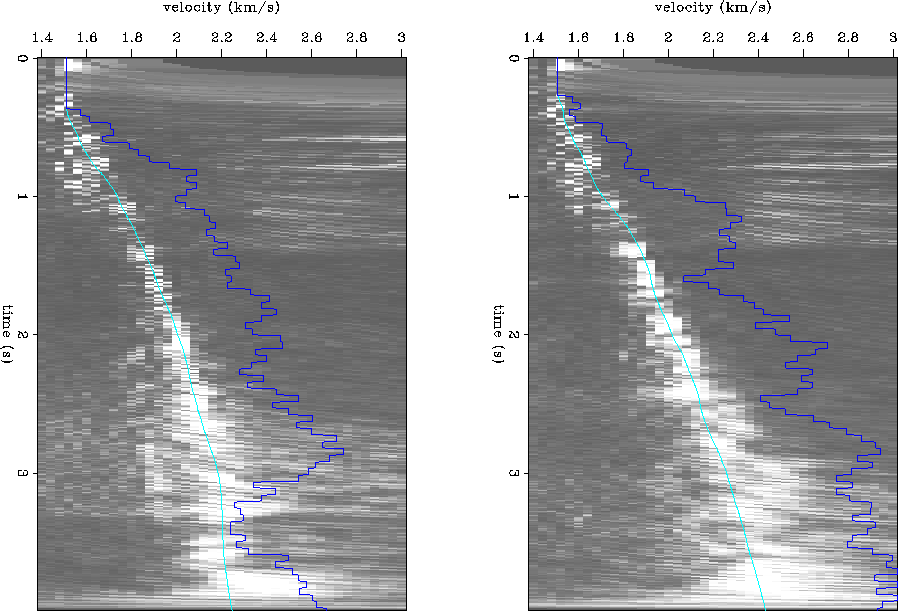
Figures ![[*]](http://sepwww.stanford.edu/latex2html/cross_ref_motif.gif) - show velocity scans and their Monte Carlo
picks, as selected at every 30 CMPs (1.0 km) along the line from the entire
survey velocity cube. One can see that the quality and shape of the
semblance peak trajectories varies along the line, and that the Monte Carlo
picks are very good in most circumstances. Note that to the east, the dipping
events are caused by the uprise of the flanks of a salt dome (which peaks just
east of 17 km at about 2 seconds depth). Some interval velocity picks
show a deep high velocity zone which may be due to the presence of salt
and/or steep dip (remember these are NMO stacking, not migration, velocities).
- show velocity scans and their Monte Carlo
picks, as selected at every 30 CMPs (1.0 km) along the line from the entire
survey velocity cube. One can see that the quality and shape of the
semblance peak trajectories varies along the line, and that the Monte Carlo
picks are very good in most circumstances. Note that to the east, the dipping
events are caused by the uprise of the flanks of a salt dome (which peaks just
east of 17 km at about 2 seconds depth). Some interval velocity picks
show a deep high velocity zone which may be due to the presence of salt
and/or steep dip (remember these are NMO stacking, not migration, velocities).
fit12
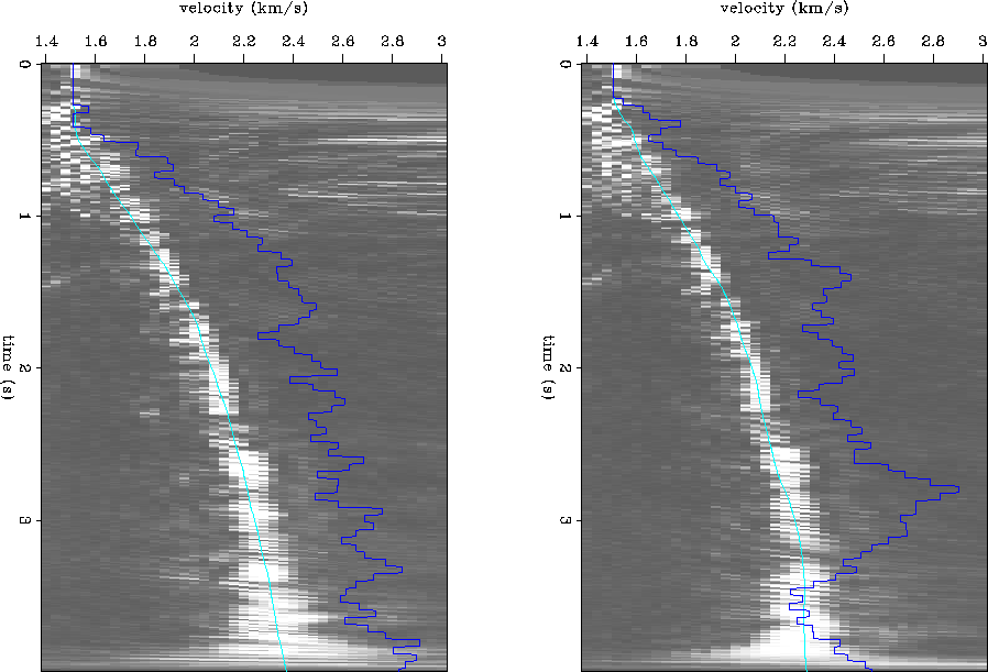
Figure 6 Velocity semblance scans at
(a) 7.0 km, and (b) 8.0 km, overlain with Monte Carlo automatic
rms and interval velocity picks.


 fit34
fit34
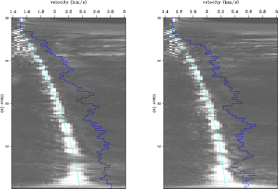
Figure 7 Velocity semblance scans at
(a) 9.0 km, and (b) 10.0 km, overlain with Monte Carlo automatic
rms and interval velocity picks.
fit56
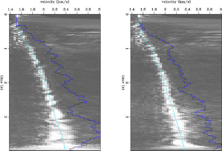
Figure 8 Velocity semblance scans at
(a) 11.0 km, and (b) 12.0 km, overlain with Monte Carlo automatic
rms and interval velocity picks.
fit78
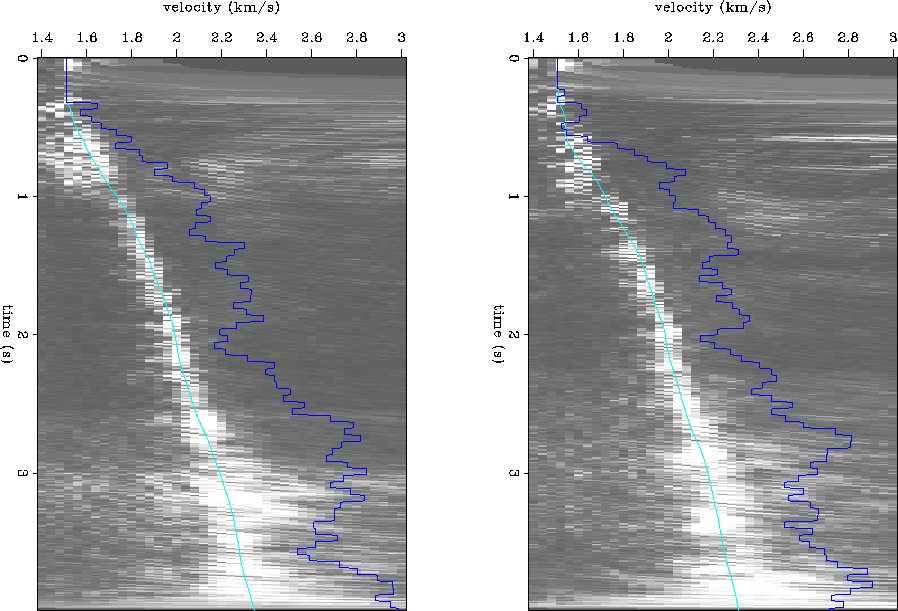
Figure 9 Velocity semblance scans at
(a) 13.0 km, and (b) 14.0 km, overlain with Monte Carlo automatic
rms and interval velocity picks.
fit90
Figure 10 Velocity semblance scans at
(a) 15.0 km, and (b) 16.0 km, overlain with Monte Carlo automatic
rms and interval velocity picks.
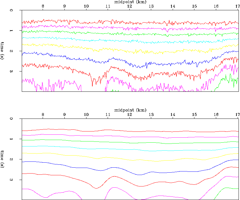
Figure shows the unsmoothed contour plot of all 300
Monte Carlo rms velocity picks in the upper panel, and the smoothed
rms velocities (a triangle of 330 m half-width) in the lower panel.
It is evident that the automatic picks exhibit a large degree of
lateral consistency, even though they are not constrained to do so.
This gives some reassurance that the Monte Carlo algorithm is somewhat
robust, at least for these 300 CMP gathers. The smoothed velocities
in Figure b are used for the subsequent Kirchhoff prestack
time migration. Note that the velocity varies laterally, and sags in
velocity toward the east where the shallow low velocity sediments have been
downthrown by the slump faults activated by the salt dome.
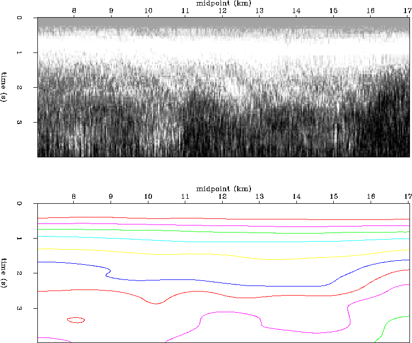
Figure shows the unsmoothed raster plot of all 300
Monte Carlo interval velocity picks, and the smoothed vi contours
below. In general, the interval velocities are much more noisy than
the rms velocities, as is to be expected. However, there is a definite
low frequency trend that parallels the rms trends and the downthrown
low velocities. This seems rather promising that there really is some
low frequency information in the interval velocities. For example,
Figure b could be used directly as a first estimate of
depth migration velocity, after a vertical time-to-depth conversion.
In fact, it would be interesting to use the smoothed interval velocity
model to convert the time migration to depth.
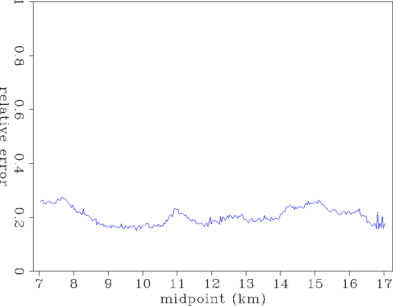
Figure is a useful byproduct of the Monte Carlo velocity
fitting procedure. It is a plot of the relative misfit error of the
velocity picks. Since the maximum possible integrated semblance value
Smax
can be calculated from each velocity scan, the relative misfit error E
measure is also available:
| 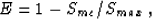 |
(5) |
where Smc is the optimal integrated semblance value that the Monte Carlo
algorithm converged to for a given velocity scan. Figure
shows that the fits are fairly consistent at about 20% relative misfit error,
which is rather good. Figure could also be extremely useful
as a Quality Control tool, since bad velocity picks will cause the error
to spike in the plot. For example, one can quickly decide that the velocity
picks around midpoints at 11 km are not as favorable as the contiguous CMP
velocity picks. For an interpreter, a quick look at this plot can tell you
(a) how good the overall picks are quantitatively, and (b) which areas
might need to be edited and repicked manually to produce the final
velocity field estimate.
mcvels
Figure 11 (a) Upper panel: unsmoothed Monte Carlo
rms velocity picks, (b) Lower panel: laterally smoothed Monte Carlo
rms velocities using a triangle of 330 m half-width.
mcvints
Figure 12 (a) Upper panel: unsmoothed Monte Carlo
interval velocity picks, (b) Lower panel: laterally smoothed
Monte Carlo interval velocities using a triangle of 330 m half-width.
mcverr
Figure 13 A plot of the Monte Carlo
velocity fit error as a function of surface midpoint coordinate.
A perfect fit would maximize semblance and represent 0.00 fit
error on the plot. A very poor fit would achieve a low semblance
integral value and represent a value near 1.00 in the fit error.
Next: Migrations
Up: A MARINE DATA EXAMPLE
Previous: Marine data and preprocessing
Stanford Exploration Project
11/17/1997