


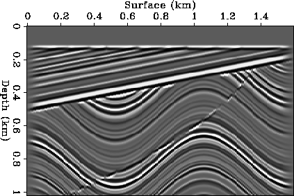
![[*]](http://sepwww.stanford.edu/latex2html/cross_ref_motif.gif) shows a synthetic reflectivity model.
A zero reflectivity layer at the top of the model represents a water layer.
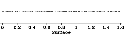
To test our resampling algorithm, we generate an unevenly sampled dataset
from this model. Figure shows the surface positions of the
receivers. The receiver spacing is randomly chosen from an uniform distribution.
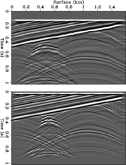
The average error in receiver position is 0.02 km, and the variance is
0.0195 km. Figure shows the zero-offset section generated
with a constant velocity of 2 km/s. The influence of the errors in
receiver position can be clearly identified. We solve the equation (2)
using the conjugate gradient method. The implementation of the Kirchhoff
upward-continuation operator is similar to the one described by Bevc (1992).
After 10 iterations, we obtain
the uniformly sampled wave field at the depth level of 0.1 km, which
is shown in Figure . It is clear that the effect of
irregular spacing has been removed by the inversion process.
Figure is a plot of the total energy of the residual as a function
the iterations of the conjugate gradient method.
Convergence is reached after 10 iterations, when the total energy of
the residual drops close to zero.
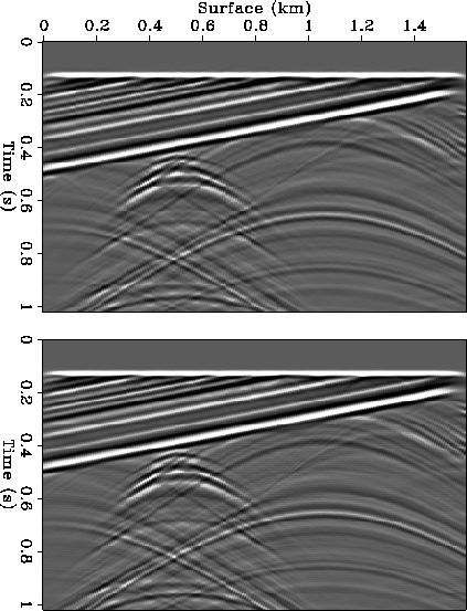
Figure displays the synthetic data resampled at surface
and the synthetic data modeled directly
from the reflectivity model for comparison. The differences are
imperceptible.
shows a synthetic reflectivity model.
A zero reflectivity layer at the top of the model represents a water layer.
To test our resampling algorithm, we generate an unevenly sampled dataset
from this model. Figure shows the surface positions of the
receivers. The receiver spacing is randomly chosen from an uniform distribution.
The average error in receiver position is 0.02 km, and the variance is
0.0195 km. Figure shows the zero-offset section generated
with a constant velocity of 2 km/s. The influence of the errors in
receiver position can be clearly identified. We solve the equation (2)
using the conjugate gradient method. The implementation of the Kirchhoff
upward-continuation operator is similar to the one described by Bevc (1992).
After 10 iterations, we obtain
the uniformly sampled wave field at the depth level of 0.1 km, which
is shown in Figure . It is clear that the effect of
irregular spacing has been removed by the inversion process.
Figure is a plot of the total energy of the residual as a function
the iterations of the conjugate gradient method.
Convergence is reached after 10 iterations, when the total energy of
the residual drops close to zero.
Figure displays the synthetic data resampled at surface
and the synthetic data modeled directly
from the reflectivity model for comparison. The differences are
imperceptible.
 |


 |
 |
|
convg
Figure 4 The total energy of the residuals of the inversion process versus the iterations of the conjugate gradient method. | 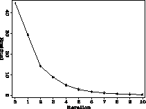 |
 |
.