The interrelation of modeling and migration

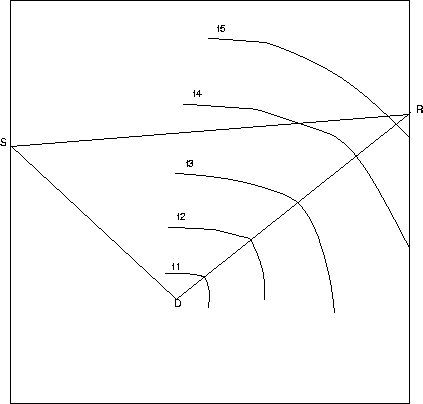
To describe modeling, let us consider the 2-D geological medium shown in Figure 1. It contains a point diffractor D in an arbitrary low-wavenumber velocity background. The recording geometry contains a source S located at one well and a series of receivers located at another well. During the modeling process, the direct wave emitted from the source S excites the diffractor D at a time equal to the minimum traveltime t_SD from the source S to the diffractor D, according to Fermat's principle. The diffractor D generates diffraction as rays DR that are recorded by the receivers. The diffraction wavefront expands from the diffractor. The direct wave SR does not pass through the diffractor D and thus does not bear information about the diffractor. The direct wave is muted before the data is input to the migration imaging process. Modeling by the finite-difference method represents the wave equation by finite-differencing. The low-wavenumber velocity background and the high-wavenumber velocity heterogeneity are represented as attributes assigned to the finite-difference grids. Each grid point is treated as a point diffractor (or secondary source). The strength of each secondary source is proportional to the reflectivity at that location. The recorded data are the history wavefields at the recording grid points (Mitchell, 1969; Alford et al., 1974; Claerbout, 1976; McMechan 1985). During the process of modeling, the low-wavenumber velocity background governs the wave propagation, and the high-wavenumber velocity heterogeneity generates the diffractions. Crosswell seismic survey is usually conducted at a subsurface segment of the well that covers the target zone; thus, during the numerical modeling process, the absorbing boundary conditions of Clayton and Engquist (1977) are applied along the four sides of the grid to simulate a whole space for wave propagation.

Migration is the process that backprojects the recorded diffraction wavefields from the recording boundary into the low-wavenumber velocity background to locate the diffractors, which constitutes of the high-wavenumber velocity heterogeneity. What is needed as additional input is a low-wavenumber velocity background model that governs the wave propagation. Migration produces the image of high-wavenumber velocity heterogeneity, that is, the locations and strengths of the diffractors. Reverse-time depth migration projects the recorded diffraction wavefields back into the low-wavenumber velocity background by taking the recorded data as boundary values of a finite-difference grid and running backward through time (McMechan, 1983). The diffraction wavefront focuses toward the location of the original diffractor. At time t_SD, all the energy that was diffracted at D will be focused at D. The value of the backpropagating wavefields at the particular grid point of D is extracted and then added as reflectivity into the image plane at the same spatial location (Chang and McMechan, 1986). As the wavefields continue to propagate backward in time, the focused energy at D defocuses and continues to backpropagate in the way each contribution originates. Each grid point is treated as a point diffractor and is imaged accordingly.

 

Geometry Figure 1 A crosswell recording geometry and demonstration of modeling and migration. During modeling, the diffraction wavefront expands from diffractor D. During reverse-time migration, the diffraction wavefront focuses toward diffractor D.