Sampling in space

This is the simplest algorithm and one that is frequently used. At each trace location the time at which the curve crosses the trace is calculated. A value for the trace at this time is then added into the integral. The value may be the value at the nearest time sample, or it may be a value interpolated from the neighboring time samples.

 

samp
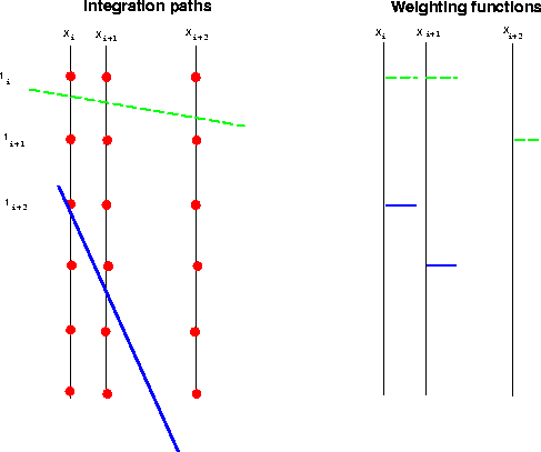
Figure 3 Sampling in space, a single sample is used at each space location. The weighting function is a set of impulses, one on each trace. Two trajectories and their corresponding weighting functions are shown. The upper, dashed, trajectory is relatively flat; the lower, solid trajectory is steep.

This method is illustrated in figure . The sample value at the trace crossing has been assigned to the region of the curve between (x_ix + x_ix-1)/2 and (x_ix+1 + x_ix)/2. Each trace is sampled at a single location. This approach can lead to operator aliasing when the dip of the summation trajectory is steep. The plot on the right of figure  shows a weighting function for each trace, the integration can be implemented by multiplying each trace by the weighting function and summing. The weighting function depends on the sampling between the traces. Since this is a space integral the weight at the sampled point will be the average distance to the neighboring traces, i.e. the spatial length of the integration path for which the sample value is used.