


The problems associated with overturned waves and initial conditions can be overcome by calculating the Green's functions in polar coordinates. Van Trier and Symes 1991 use polar coordinates for similar reasons in their finite difference solution to the eikonal equation.
I will follow exactly the same steps in deriving the algorithms in polar coordinates as I did in rectangular coordinates. In a 2-D polar coordinate frame, the wave equation is,
![]()
![]()
| P(r) = P(r0) e i kr ( r- r0 ) , | (2) |
![]()
![]()
The initial conditions are not supplied at r=0, but rather at some finite initial radius r0. The region between the origin and r0 is assumed to be homogeneous. A suitable initial condition is,
![]()
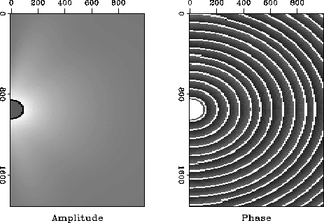
Figure ![[*]](http://sepwww.stanford.edu/latex2html/cross_ref_motif.gif) shows the amplitude and phase plots for a mono-frequency
Green's function calculated for a constant velocity medium. The polar
coordinate data has been re-interpolated onto the same rectangular grid as
the rectangular coordinate data. The amplitude is now more
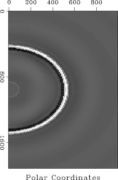
uniform for all dips. Figure shows one time slice through
the full Green's function in the (x,z,t) domain. The result is a much more
accurate representation of the wavefront.
shows the amplitude and phase plots for a mono-frequency
Green's function calculated for a constant velocity medium. The polar
coordinate data has been re-interpolated onto the same rectangular grid as
the rectangular coordinate data. The amplitude is now more
uniform for all dips. Figure shows one time slice through
the full Green's function in the (x,z,t) domain. The result is a much more
accurate representation of the wavefront.
 |


 |