Next: Real data example
Up: Introduction
Previous: Introduction
A simple 2-D example serves to demonstrate the different
methods and their noise suppression capabilities.
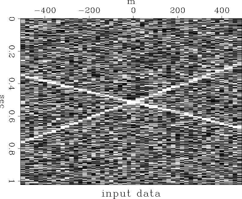
Figure ![[*]](http://sepwww.stanford.edu/latex2html/cross_ref_motif.gif) shows a synthetic dataset containing
two dipping events. Random noise with a signal to noise
amplitude ratio of 1:1 has been added.
shows a synthetic dataset containing
two dipping events. Random noise with a signal to noise
amplitude ratio of 1:1 has been added.
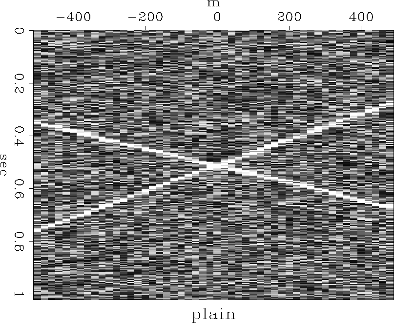
In Figure , the straightforward 3-D interpolation
scheme of SEP-73 is applied. For each output location,
we select the N (here N=15) nearest neighbors. Each pair of
traces is cross-correlated, and the results are combined to give
an estimate of event coherency as a function of dip. The dip
which gives the maximum coherency is chosen, and the traces
are summed along this trajectory to give a new trace at the
desired output location. Although the stack is over fifteen
traces, the noise has not been attenuated significantly.
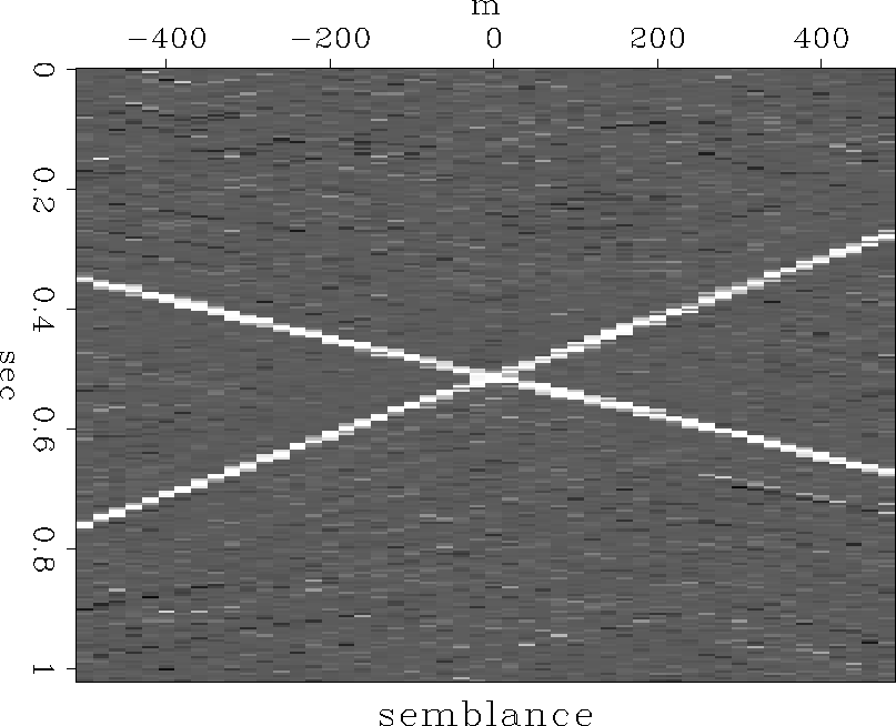
In Figure , the stack is weighted by the coherency,
computed as a function of time, measured along the best dip
direction. (Actually semblance is being used here instead of the
generalized coherency of SEP-73.)
This weighting supplements the noise suppression
power of the stack and makes a cleaner result. In Figure ,
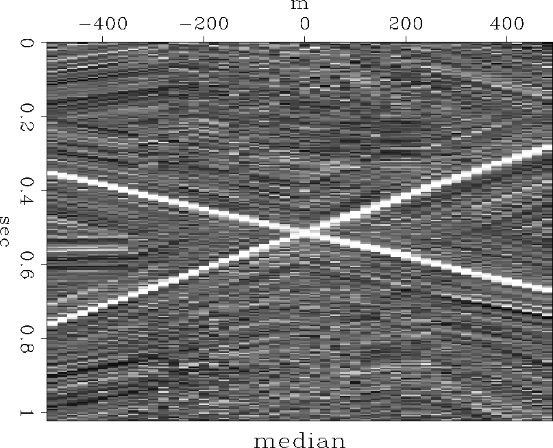
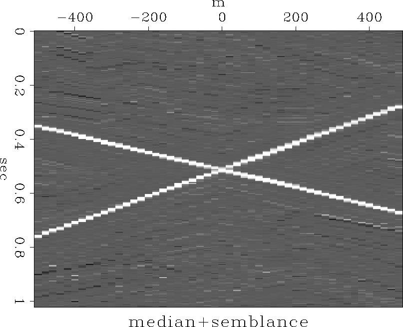
the median is used instead of the mean, and in Figure ,
both the median and semblance weight are used. This combination
gives the best overall noise suppression.
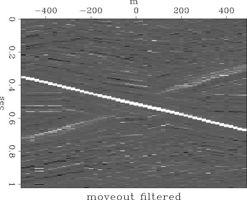
An example of velocity filtering is shown in Figure .
Here we have limited the algorithm to scan over only a certain
range of dips; the more steeply dipping event is filtered out.
Note that this method does not attempt to deal with the problem
of aliased energy.
noise
Figure 1 Synthetic example containing two dipping events. Random noise has been added with a signal to noise ratio of 1:1.


 interp
Figure 2 Synthetic interpolated to same geometry to test noise suppression properties. No semblance weighting has been applied, and the mean is used for stacking, so there is little noise suppression.
semb
Figure 3 Semblance weighting has been applied.
med
Figure 4 Median filter has been applied along the best dip trajectory, rather than the mean of conventional stacking.
medsemb
Figure 5 Both median and semblance weighting used.
filt
Figure 6 A velocity filtering example. Limiting
the range of dips searched by the algorithm can attenuate other dips.
Next: Real data example
Up: Introduction
Previous: Introduction
Stanford Exploration Project
11/17/1997