

Next: CONCLUSIONS
Up: Biondi and van Trier:
Previous: Pan_Zoom
An important reason for having chosen AVS as the software platform
to develop our seismic data visualizer is that within
AVS seismic data can be easily displayed together with other
geophysical data.
For example a 3-D dataset can be rendered together
with a surface representation of the geological
structures by merging the display of our visualizer
with the display of a geological modeling program (e.g. GOCAD).
Another useful application is to display a velocity
model together with a 3-D seismic dataset.
The AVS rendering module geometry viewer is the basic tool that
can be used to integrate the display of different
geophysical data. It can render in the same view multiple
3-D geometries, each of which can describe seismic data, velocity
models, or geological models.
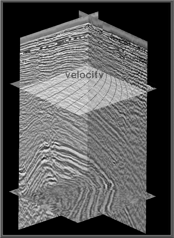
Figure ![[*]](http://sepwww.stanford.edu/latex2html/cross_ref_motif.gif) shows an example of a combined display
of 3-D seismic data with a 3-D velocity function.
The data and the velocity model are independently sliced,
the slices are then rendered in a three-dimensional space
and displayed in the same view.
To facilitate the interpretation of the display,
a contour plot of the velocity model is superimposed to the
velocity slice, and two different colormaps
are used for color-coding the velocity model and the
seismic data.
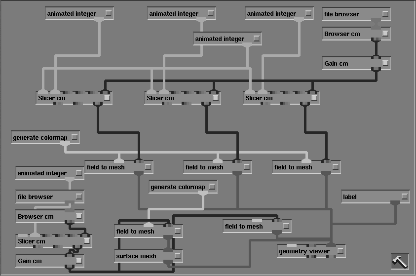
Figure 8 shows the CM/AVS network we used to generate the
display in Figure
shows an example of a combined display
of 3-D seismic data with a 3-D velocity function.
The data and the velocity model are independently sliced,
the slices are then rendered in a three-dimensional space
and displayed in the same view.
To facilitate the interpretation of the display,
a contour plot of the velocity model is superimposed to the
velocity slice, and two different colormaps
are used for color-coding the velocity model and the
seismic data.
Figure 8 shows the CM/AVS network we used to generate the
display in Figure ![[*]](http://sepwww.stanford.edu/latex2html/cross_ref_motif.gif) .
The seismic data are read, gained, and sliced on the CM-5, and then
passed to the AVS module field to mesh that generates 3-D geometries
that are finally rendered and displayed by the geometry viewer module.
Similarly, the velocity model is read, sliced, and gained on the CM-5,
before being rendered together with the data by geometry viewer.
Although the rendering is limited to 3-D geometries,
the capability of our CM/AVS modules to manage datasets
with higher dimensionality than three can be exploited
by stepping in time along the other axes.
For examples, the data shown in Figure
.
The seismic data are read, gained, and sliced on the CM-5, and then
passed to the AVS module field to mesh that generates 3-D geometries
that are finally rendered and displayed by the geometry viewer module.
Similarly, the velocity model is read, sliced, and gained on the CM-5,
before being rendered together with the data by geometry viewer.
Although the rendering is limited to 3-D geometries,
the capability of our CM/AVS modules to manage datasets
with higher dimensionality than three can be exploited
by stepping in time along the other axes.
For examples, the data shown in Figure ![[*]](http://sepwww.stanford.edu/latex2html/cross_ref_motif.gif) are the results
of many 3-D poststack migrations merged together along the
fourth axes of the dataset.
The migrations were obtained using different
filters for the Hale-McClellan algorithm
Biondi and Palacharla (1993); Palacharla and Biondi (1993).
The quality of the results can be easily compared by
switching between different migrations by slicing
the 4-D dataset along the fourth axis.
are the results
of many 3-D poststack migrations merged together along the
fourth axes of the dataset.
The migrations were obtained using different
filters for the Hale-McClellan algorithm
Biondi and Palacharla (1993); Palacharla and Biondi (1993).
The quality of the results can be easily compared by
switching between different migrations by slicing
the 4-D dataset along the fourth axis.
3d-geo-disp-vel
Figure 7 Integrated display of a 3-D seismic dataset together with a 3-D
velocity function. A contour plot of the velocity slice is
superimposed to the rendering of the slice itself.
 3d-geo-net-vel
Figure 8 CM/AVS network for displaying a 3-D dataset together
with a velocity model.


Next: CONCLUSIONS
Up: Biondi and van Trier:
Previous: Pan_Zoom
Stanford Exploration Project
11/16/1997
![[*]](http://sepwww.stanford.edu/latex2html/cross_ref_motif.gif) shows an example of a combined display
of 3-D seismic data with a 3-D velocity function.
The data and the velocity model are independently sliced,
the slices are then rendered in a three-dimensional space
and displayed in the same view.
To facilitate the interpretation of the display,
a contour plot of the velocity model is superimposed to the
velocity slice, and two different colormaps
are used for color-coding the velocity model and the
seismic data.
Figure 8 shows the CM/AVS network we used to generate the
display in Figure
shows an example of a combined display
of 3-D seismic data with a 3-D velocity function.
The data and the velocity model are independently sliced,
the slices are then rendered in a three-dimensional space
and displayed in the same view.
To facilitate the interpretation of the display,
a contour plot of the velocity model is superimposed to the
velocity slice, and two different colormaps
are used for color-coding the velocity model and the
seismic data.
Figure 8 shows the CM/AVS network we used to generate the
display in Figure ![[*]](http://sepwww.stanford.edu/latex2html/cross_ref_motif.gif) .
The seismic data are read, gained, and sliced on the CM-5, and then
passed to the AVS module field to mesh that generates 3-D geometries
that are finally rendered and displayed by the geometry viewer module.
Similarly, the velocity model is read, sliced, and gained on the CM-5,
before being rendered together with the data by geometry viewer.
Although the rendering is limited to 3-D geometries,
the capability of our CM/AVS modules to manage datasets
with higher dimensionality than three can be exploited
by stepping in time along the other axes.
For examples, the data shown in Figure
.
The seismic data are read, gained, and sliced on the CM-5, and then
passed to the AVS module field to mesh that generates 3-D geometries
that are finally rendered and displayed by the geometry viewer module.
Similarly, the velocity model is read, sliced, and gained on the CM-5,
before being rendered together with the data by geometry viewer.
Although the rendering is limited to 3-D geometries,
the capability of our CM/AVS modules to manage datasets
with higher dimensionality than three can be exploited
by stepping in time along the other axes.
For examples, the data shown in Figure ![[*]](http://sepwww.stanford.edu/latex2html/cross_ref_motif.gif) are the results
of many 3-D poststack migrations merged together along the
fourth axes of the dataset.
The migrations were obtained using different
filters for the Hale-McClellan algorithm
Biondi and Palacharla (1993); Palacharla and Biondi (1993).
The quality of the results can be easily compared by
switching between different migrations by slicing
the 4-D dataset along the fourth axis.
are the results
of many 3-D poststack migrations merged together along the
fourth axes of the dataset.
The migrations were obtained using different
filters for the Hale-McClellan algorithm
Biondi and Palacharla (1993); Palacharla and Biondi (1993).
The quality of the results can be easily compared by
switching between different migrations by slicing
the 4-D dataset along the fourth axis.

