3-D prestack depth migration: Why Kirchhoff?

François Audebert

Author has no known email address

ABSTRACT

3-D prestack depth migration is emerging as an industrial imaging tool. Many competing algorithms have been proposed by various authors. Nevertheless, the real bottleneck in 3-D prestack processes is the sheer amount of input and output data. This paper reviews the principal migration methods on the basis of their capacity for data manipulation, without evaluating the algorithms themselves. It concludes that Kirchhoff methods are the best first candidates, while other methods dealing with subsets of input data may have to be taken into account in the future.

Prestack depth migration in three dimensions is expected to become a routinely available imaging tool within a few years. Many authors have already formulated algorithms: Wapenaar et al. (1986); implementations: Lumley and Biondi (1991), Cabrera et al. (1992), Cao (1992); and even real-case experiments: Western and Ball (1992), Ratcliff (1993), to mention but a few names.

Nevertheless, 3-D prestack migration is an expensive tool, whatever algorithms are used. The immediate priority is to reach feasibility, first with simplistic algorithms; refinements will follow in due time. The fundamental hindrance is not the mathematical complexity of the data processing involved; it is the huge amount of data. The massive amounts of data saturate present-day capacities for number crunching, memory space and input/output management. Technologies evolve, but at very different rates: for instance, computer power increases much faster than input/output speed or memory capacity. Hardware characteristics set the rules with respect to software development. As a consequence, the strategy of data management is of paramount importance.

The goal of this review is to categorize the existing or potential 3-D prestack migration methods, on the basis of their abilities to manipulate data.

THE HEAVY COSTS OF MIGRATION

The 3-D post stack migration of a big survey, performed with explicit finite-difference algorithms saturates both the memory and the CPU capacity of the most powerful existing machines.

Migration versus machine capacities

As of today, the post-stack migration of large 3-D surveys, with the most sophisticated imaging tools, may exceed the capacity of the available machines. A typical sophisticated post-stack imaging method would be a 3-D explicit finite-difference migration. It must be 3-D, because Earth is now acknowledged, in the seismic processing industry, to be three-dimensional. It must be a finite-difference code, because such codes are efficient at handling amplitudes in variable velocity media. And finally, explicit operators, such as Hale-McClellan, Hale (1991), or Remez-Soubaras, Soubaras (1992), are recommended for the sake of numerical azimuthal isotropy.

In the post-stack case, the original 3-D data are already stacked; a significant condensation of data has been done. Moreover, the finite-difference algorithms work in the $(\omega,x,y)$ domain, and frequency slices can be processed independently. Thus a smaller volume of data, with respect to the volume of the prestack survey, is actually present at any given time in the machine. In spite of this enormous condensation of data volume, both the I/O capacity and the memory capacity of the today's biggest existing machines are stretched to the limit, even for less than gigantic 3-D surveys. Today, the CPU time required for a large survey is on the order of days. This is problematic considering the conventional wisdom that a process requiring one to several weeks of CPU time is not realizable, at least as a routine process.

In the sections that follow, I take this most sophisticated 3-D post-stack migration as a standard of comparison and the unit of feasibility. In comparison, any 3-D prestack migration will then take several orders of magnitude more time and resources, simply because the amount of input data is several orders of magnitude larger.

Not all 3-D prestack strategies are equivalent. Any prestack migration process deals with some kind of subset of data at a time; the subsets differ depending on the strategy adopted. Moreover, some strategies may be more efficient, for instance, at not handling unnecessary zeroes or at avoiding multiple access to input data.

It is the aim of this study to compare on a common reference basis those different strategies. I intentionally refer here to migration strategies rather than migration methods or algorithms, because the comparison concerns the strategies of handling the data, not internal algorithmical or mathematical aspects.

Typical figures for an average 3-D survey

From seismic acquisition and processing, one can extract an average pattern for a 3-D survey, shown on Figures cube3 and  cube4.

 

cube3
Figure 1 The global image volume N_x * N_y * N_z of a 3-D survey , and the subvolume M_x * M_y * Nz illuminated by a shot experiment.

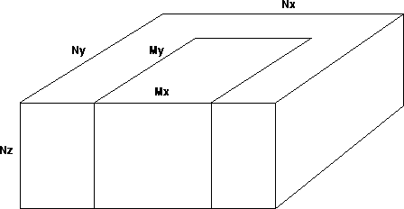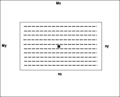
The key parameters for the input traces are the number of shots N_S, the number of receivers per shot N_g, and the number of time samples per trace N_t. The key parameters for the survey pattern are, 1) the number of bins in the X and Y directions, N_X and N_Y, which corresponds to the midpoint dimension, and 2) the maximum extent in X and Y of a common shot array, expressed in number of bins, n_x and n_y, which corresponds to the offset dimension. Finally, an additional key parameter for migration is the extension in depth of the velocity model and the output image:
N_Z depth steps at the scale of the velocity grid. All important figures and volumes of the 3-D survey can be expressed with these parameters.

 

cube4
Figure 2 The surface extension of a common shot array, n_x * n_y, and the surface extension of the illuminated volume, M_x * M_y.

This paper uses the following conventions:
1) the solid brackets [ ] enclose fundamental or unsplittable quantities, as in [ N_X N_Y ];
2) products without a separating asterisk * indicate homogeneous volumes, as in N_X N_Y where N_X and N_Y are interchangeable;
3) products with a separating asterisk * indicate the product of heterogeneous quantities, as in $N_{\omega}$ * [ N_X N_Y ] where $N_{\omega}$ is a number of frequency slices and [ N_X N_Y ] is the size of one slice;
4) the parentheses ( ) will denote an intermediate hierarchy of processes or subsets.

Finally, the typical magic numbers are as follows.

• Acquisition data

  $\bullet$

  Number of shots $N_S \approx 2.5 * 10^4$.

  $\bullet$

  Number of traces per shot $N_g \approx 5 * 10^2$.

  $\bullet$

  Trace length $N_t \approx N_\omega \approx 10^3$.
  The number of samples for the input traces is approximately the same in the time and frequency domains.

  $\bullet$

  Total acquisition data volume = $N_S * N_g * N_t \approx 12.5 * 10^9$.
  These are the data recorded in the field, the total number of traces times the number of samples per trace.

• Gridding of the survey:

  $\bullet$

  Grid size (surface) = $N_X * N_Y \approx 10^6$.
  This is the total number of bins of the survey, with $N_X \approx N_Y \approx 10^3$.

  $\bullet$

  Grid size in depth = $N_Z \approx 10^2$.
  This is the number of extrapolation steps; the number of samples in depth of the image is $\approx N_Z * 10$.

  $\bullet$

  Area covered by a common-shot array = $n_x n_y \approx 10^3$.
  This is the area covered by a 3-D shot gather, in number of bins.

  $\bullet$

  Illumination window of a shot = $M_X * M_Y \approx 10^4$.
  This is the projection at the surface of the volume actually illuminated by a shot experiment, expressed in number of bins.

• Auxiliary volumes

  $\bullet$

  Total velocity model = $N_X * N_Y * N_Z \approx 10^8$.

  $\bullet$

  Traveltime volume for one source = $M_X * M_Y * N_Z \approx 10^6$.

  $\bullet$

  Total traveltime volume = $N_X * N_Y * [ M_X * M_Y * N_Z ] \approx 10^{12}$.
  This is the volume illuminated by a shot experiment, times the number of surface locations.

THE REFERENCE MIGRATION

On this average representative 3-D survey, the last step of standard seismic processing would be today the most sophisticated 3-D post-stack migration available.

An explicit finite-difference method of 3-D post-stack migration

The reference 3-D post-stack migration I have chosen is a frequency-space, explicit finite-difference method. Though I have selected a specific migration method, it is quite representative with regard to data-wise strategy. The situation would be nearly identical for any post-stack frequency-space or frequency-wavenumber algorithm such as the Stolt, phase-shift, PSPI, split-step algorithm. The only difference would be the value of an atomic algorithm-dependent factor. In the remainder of this paper, the algorithm factor for post-stack is represented by a coefficient K₁, and the prestack algorithm factor by the coefficient K₂. The algorithm factor for Kirchhoff algorithm, is generally different, and is represented here by the coefficient K₂. As previously specified, the quantity between solid brackets [ ] represents a irreducible, non-splittable, basic unit of data.

$\bullet$ INPUT = $N_\omega * [ N_X N_Y ]$
There are $N_{\omega}$ independent frequency slices, each of size N_X * N_Y.

$\bullet$ MEMORY = $N_\omega * [ N_X N_Y ]$ + output + velocity model.
There are, at any given time in memory at least one of the $N_{\omega}$ frequency slices, plus the output volume (the migrated image), plus the velocity model.

$\bullet$ CPU COST = $K_1 * N_\omega * [ N_Z * N_X N_Y ]$
The cost is an approximately linear function (for high values) of the size of the frequency slices processed, and a linear function of the number of frequencies processed.

In the average 3D, one has: $N_X \approx N_Y \approx 10^3$, $N_\omega \approx 10^3$, and $N_Z \approx 5 * 10^2$.

Nevertheless, this study does not concern the absolute values of input size, memory requirement, and computation cost. I only use them as a standard for comparison.

3-D SG MIGRATION

SG migration is a favourite prestack migration in two dimensions. It is legitimate to think of its extension to three dimensions.

An explicit finite-difference method of 3-D SG migration

An SG migration by an explicit finite-difference algorithm would be the ultimately perfect method of 3-D prestack migration, if it were available. It would combine the good behaviour of 2-D SG migration in complex velocity model, with the good numerical isotropy of the zero-offset migration by explicit finite-difference operators (preceding section). Algorithmically speaking, it is identical to its zero-offset (= post-stack) equivalent I have described in the preceding section, but with extra offset dimensions. Every bin of the zero-offset case is the site of a virtual shot, with a two-dimensional regular receiver array centered on the bin. This virtual regular receiver array should include the largest common-shot arrays and common-receiver arrays of the survey. The SG migration is based on alternated downward continuations of common-shot gathers and downward continuations of common-geophone gathers. The downward continuation of a common-shot gather or a common-geophone gather is very similar to the downward continuation of zero-offset data, all surface dimensions being equal.

$\bullet$ INPUT = $N_\omega * [ N_X N_Y * n_x n_y ]$
Each of the $N_{\omega}$ frequency slices can be processed separately.

$\bullet$ MEMORY = $N_\omega * [ N_X N_Y * n_x n_y ]$ + output + velocity model

$\bullet$ CPU COST = $K_2 * N_\omega * [ N_Z * ( N_X N_Y * n_x n_y ) ]$

Typically $( n_x n_y ) \approx 10^3$

Performance ratio with respect to 3-D post-stack migration

To obtain the performance ratio, I divide the cost and volume by those of the reference 3-D post-stack migration.

$\bullet$ MEMORY: $( n_x n_y ) \approx 10^3$ to 10⁴

$\bullet$ CPU COST: ${K_2 \over K_1}$ * ( n_x n_y) $\approx {K_2 \over K_1 } * ( 10^3$ to 10⁴ )

The ratio ${K_2 \over K_1}$ may be as low as 2, but even in this most favorable case, one is left with four orders of magnitude beyond the present feasibility threshold. The figures are similar, except for the value of the coefficient K₂, for 3-D prestack Stolt, phase-shift, PSPI, split-step, and others frequency-space or frequency wavenumber algorithms. Three-dimensional SG Kirchhoff migration is not considered here, because simulating downward continuation with Kirchhoff methods is comparatively very costly and inefficient.

Clearly, SG migration in three dimensions is not feasible for the near future. There are four orders of magnitude to gain, which requires many more years of technical progress.

3-D SHOT-PROFILE MIGRATION

Shot-profile migration is commonly used in two dimensions, in the implicit finite-difference implementation, as an alternative to SG migration.

A finite-difference method of 3-D shot-profile migration

In this migration method, each shot-gather is processed separately. Each shot-gather is migrated into an illuminated volume M_X M_Y N_Z, smaller than the whole image volume, but bigger than the simple vertical prolongation of the area covered by the shot-array. The shot-profile migration is very similar to a zero-offset migration done twice into the same illuminated volume. Twice, because for every depth step there is a source-wavelet extrapolation followed by a receiver wavefield extrapolation, where each of these extrapolations is pretty similar to a zero-offset extrapolation, both from the algorithmic and the data point of view.

$\bullet$ INPUT = $N_S * ( N_\omega * [ M_X M_Y ] )$
All shot-gathers are processed independently, and for a given shot-gather each frequency slice may be processed separately.

$\bullet$ MEMORY = $N_S * ( N_\omega * [ M_X M_Y ] )$ + output + velocity model

$\bullet$ CPU COST = $K_2 * N_S * ( N_\omega * N_Z * [ M_X M_Y ] )$

with typically: $M_X \approx M_Y \approx 10^2$ , $N_S \approx 2.5 * 10^4$, $N_g \approx 5 * 10^2$ .

Performance ratio with respect to 3-D post-stack migration

The following performance ratio are the aforementioned memory requirements and CPU costs compared to their 3-D post-stack equivalents.

$\bullet$ MEMORY: N_S * ( M_X M_Y ) / $( N_X N_Y ) \approx N_S * 10^{-2}$

$\bullet$ CPU COST: ${K_2 \over K_1} * N_S * ( M_X M_Y )$ / $( N_X N_Y ) \approx {K_2 \over K_1} * 2.5 * 10^2$

The memory and cost ratios ( 10^-2 and 10³) become more favorable than in the case of SG migration ( 10⁴ and ${K_2 \over K_1} * 10^4$ respectively). Undoubtedly, each shot-gather would fit in memory. But still, as a matter of total cost, this method is three orders of magnitude beyond feasibility. Another negative factor is that an individual shot-migrated image is a very bad partial image, with many edge effects and illumination artifacts, thus hard to interpret and nearly useless. The artifacts can generally be suppressed by stacking a sufficient numbers of partial images, but to do so one needs to migrate as much as one-fourth of the total shots of the survey. One-fourth of the total survey is not an affordable subset to produce a first ``cheap'' legible partial image.

3-D PLANE-WAVE MIGRATION

The decomposition of seismic data into plane-wave or common-angle dataset, by such operations as slant-stack or Tau-P transform, is frequent if not standard practice. In three dimensions, some research is done on Tau-P migrations, but more publicised are plane-wave and areal-source migrations in the frequency-space domain. Areal-source migration is closely related to plane-wave migration.

Three dimensional plane-wave migration in the frequency-space domain

The interest in plane-wave migration is that, for each plane wave, the data volume is equivalent to a zero-offset data volume. Consequently, with regard to memory and space, there is no doubt that one plane-wave migration would fit in the machine. Because of the similarity of volume, and the intrinsic parallelism between plane-wave and zero-offset algorithms, the cost of one plane-wave migration is almost the same as the cost of the post-stack migration with equivalent implementation.

Qualitatively, a plane-wave experiment provides a fairly regular illumination of the subsurface. The migration of one plane wave yields a generally coherent, legible, and artifact-free image of the subsurface, very similar in that respect to a zero-offset image. Except for eventual signal-to-noise ratio problems, it is quite an acceptable partial image.

But a few important points are to be clarified. The extra cost of plane-wave synthesis has to be assessed. It is difficult and debatable to evaluate the number of plane waves that would be needed to produce a satisfactory final output migrated image. The range is from 20, for a minimalist selection of dip and azimuth in three dimensions, to more than 100, for regular illumination, though the figures are debatable.

$\bullet$ INPUT = $N_{PW} * ( N_\omega * [ N_X N_Y ] )$

$\bullet$ MEMORY = $N_{PW} * ( N_\omega * [ N_X N_Y ] )$ + output + velocity model

$\bullet$ CPU COST = $K_1 * N_{PW} * ( N_\omega * N_Z * [ N_X N_Y ] )$ + plane-wave synthesis

with typically $N_{PW} \approx 20 - 100$

Performance ratio with respect to 3-D post-stack migration

The performance ratio reduces to the number of plane waves needed.

$\bullet$ MEMORY: $N_{PW} \approx 20 - 100$

$\bullet$ CPU COST: $N_{PW} \approx 20 - 100$ (without counting plane-wave synthesis)

Given the number of plane waves I deemed necessary, the feasibility diagnosis looks good; memory space is not a problem, and the CPU cost is only two orders of magnitude beyond the reference threshold. Nevertheless, this method is not feasible in the near future because of the cost of plane-wave synthesis, and the enormous shuffling of data it involves. Unfortunately, the synthesis of one plane wave requires browsing all the input prestack data. Since huge amounts of data should not be accessed repetitively, the procedure is impractical.

3-D COMMON-OFFSET AND COMMON AZIMUTH MIGRATION

With common-offset migration, one is normally entering the world of the Kirchhoff migration. So far, common-offset migration has been only possible with Kirchhoff type implementation. Nevertheless, some research is done on frequency-wavenumber implementations of common-offset migration, (), and common-azimuth migration, (). In this section, I discuss the data aspects of these potential frequency-wavenumber implementations. The Kirchhoff implementations are discussed further on in this paper.

Common-offset gathers

The common-offset sorting of data has the advantage that it is natural: unlike a plane-wave gather, a common-offset gather exists in the input data. Creating a common-offset gather is just a matter of sorting, and it is actually frequently done in standard processing.

Another interesting feature is that common-offset data are pretty much comparable to zero-offset or post-stack data, in terms of size and spatial extension. That is to say, first, a common-offset migration should be no more expensive than a post-stack migration, and second, a constant offset migrated section is the best possible partial migration (even with respect to plane-wave migration, and a fortiori with respect to shot-profile migration). The reason is that a common-offset gather ensures a fairly good regular illumination of the subsurface. Generally, except for signal-to-noise ratio, a constant offset migrated image exhibits few artifacts and looks much like the final stacked image.

The concept of offset, and common-offset sorting, is straightforward in two dimensions, but in three dimensions it needs to be clarified. The 3-D offset has in fact two dimensions: 1) the radius or absolute offset, i.e. the absolute shot-receiver distance, and, 2) the azimuth of the shot-receiver direction. For simplicity, I designate as common-offset data, data that have same absolute offset and same azimuth. With regard to data volume, a common-offset gather is comparable to a zero-offset or post-stack dataset.

Non-Kirchhoff 3-D common-offset migration

As already mentioned, the Kirchhoff implementations are discussed further in this paper. The figures I present here are for a purely hypothetical F-X implementation, where the fictitious common-offset migration would be ``fold'' times a zero-offset migration, in terms of volume and cost.

$\bullet$ INPUT = fold * N_t * [ N_X N_Y ],
where ``fold'' is the number of traces per bin, a bin being defined by a
doublet (absolute offset, azimuth).

$\bullet$ MEMORY = fold * N_t * [ N_X N_Y ] + image + velocity model

$\bullet$ CPU COST =$K_1 * N_{\alpha} N_h *$ ( fold * [ N_Z * N_X N_Y ])
where $N_{\alpha}$ is the number of azimuths, N_h is the number of absolute offsets, and $N_{\alpha} N_h *$fold is of the order of the total number of traces N_S N_g. I have no figure estimate for $N_{\alpha}$ or N_h.

Performance ratio: 3-D common-offset and 3-D post-stack migrations

The figures are for a purely hypothetical F-X implementation, and thus they are only speculative.

$\bullet$ MEMORY= fold $\approx 1$ (number of traces per offset, per azimuth)

$\bullet$ CPU COST= $N_{\alpha} * N_h$ , the number of azimuths and offsets in which the prestack data has been redistributed, I have no figure estimate.

Non-Kirchhoff common azimuth migration

Common azimuth migration is very closely related to the previously described common-offset migration. As discussed in the preceding section, a common-offset gather is made of traces having both the same common absolute offset and the same common azimuth. A common-azimuth subset of data encompasses all absolute offsets for a given azimuth. For example, the subset can be composed of parallel 2-D acquisition lines. Thus a common-azimuth migration is the generalisation of the migration of a 2-D acquisition line in a 3-D volume. In the case of a mono-streamer marine acquisition, with no feathering of the cable, the whole survey is one common-azimuth gather. In this case, the common-azimuth migration suffices for the entire prestack migration. Here are two reasons for separating common-azimuth migration from common-offset migration. One is that common-azimuth migration seems no longer to be an exclusive Kirchhoff fiefdom: a companion paper, (), describes a possible common-azimuth migration with both Stolt and phase-shift algorithms. Secondly, common-azimuth migration produces a highly acceptable partial image: regular illumination, high fold, and relative insensitivity to azimuthal anisotropy of velocities. The following figures are tentative estimates for a F-K or F-X implementation.

$\bullet$ INPUT = N_h * fold $* N_{\omega} * [ N_X N_Y ]$,
where ``fold'' is the number of traces per bin, a bin being defined
by a doublet (absolute offset, azimuth)

$\bullet$ MEMORY = N_h * fold $* N_{\omega} * [ N_X N_Y ]$ + image + velocity model.

$\bullet$ CPU COST =$K_1 * N_{\alpha} * [ N_h * ( N_Z * N_X N_Y ) ]$,
where $N_{\alpha}$ is the total number of azimuths, N_h is the number of absolute offsets per azimuth. $N_{\alpha} * N_h$ is about the number of input traces N_S N_g.

Performance ratio: 3-D common-azimuth and 3-D post-stack migrations

$\bullet$ MEMORY: N_h * fold $\approx 10^2$?

$\bullet$ CPU COST: $N_{\alpha} * N_h \approx 10^3 ?$

3-D KIRCHHOFF PRESTACK MIGRATION

From the point of view of data-management, all Kirchhoff methods are identical: they can have any subset in input or in output.

A Kirchhoff migration is a trace by trace migration

A Kirchhoff migration can accept as input any subset of data, and as output any local or global target image. It operates truly trace by trace, thus allowing common-offset or common-shot migration. This latter implementation is the most frequent; it is the Kirchhoff version of the finite-difference shot-profile migration described earlier in this paper. The output volume is the same, but the handling of input data is different. As with finite-difference shot-profile migration, the output can be limited to the subsurface volume actually illuminated by the considered shot. In the Kirchhoff implementation, each trace of the shot-gather is ``exploded'' over the image volume, according to pre-computed traveltimes or Green's functions.

$\bullet$ INPUT = N_S N_g N_t,
no more and no fewer than the total number of traces of the survey.

$\bullet$ MEMORY = ad hoc number of traces + image + traveltime tables,
we can process as many traces at a time as we want, starting from one.

$\bullet$ CPU COST = K₃ * N_S N_g * [ N_Z * ( M_X M_Y ) ] + traveltime computation.
The coefficient K₃ is the algorithm factor of Kirchhoff methods. The number of time samples per input trace N_t the number of time samples per input trace does not appear in the computation cost. In Kirchhoff methods, the computation cost is just proportional to the number of input traces, times the volume of the output image.

Performance ratio with respect to 3-D post-stack migration

Due to the very different features of Kirchhoff and finite-difference migration, a performance ratio with respect to the reference 3-D post-stack migration is not easy to quantify.

$\bullet$ MEMORY:
(1 trace + 1 traveltime table)
to compare to
(1 frequency slice + 1 velocity cube).
The ratio is about 10^-2.

$\bullet$ CPU COST: ${K_3 \over K_1} * N_S N_g * ( M_X M_Y )$ / ( N_X N_Y ) $\approx {K_3 \over K_1} * 1.5 * 10^3$,
not accounting for traveltime computation.

COMPARATIVE FEATURES OF KIRCHHOFF AND OTHER APPROACHES

Kirchhoff and other approaches have very different nature and characteristic. It is a fact to be taken seriously into consideration in this comparative study. The differences are in the ``invisible'' auxiliary processing, often taken for granted, and in the factors affecting the memory requirements and the cost.

Auxiliary processing

The auxiliary processings are prerequisites to the migration process, assumed done beforehand, like Fourier transform, plane-wave synthesis or any sorting of data. It is important to keep in mind that most if not all migration methods involve some side processing, and the overhead costs incurred may not be negligible. Kirchhoff migrations require a prior traveltime or Green's function computation, and all frequency-space migrations require a previous Fourier transform of the input data (several Fourier transforms for the frequency-wavenumber algorithms).

Minimum memory requirement

This section compares now the absolute minimum working volumes of Kirchhoff and frequency-space migration.

*

The minimum volume for a prestack Kirchhoff migration comprises

$\bullet$

a source+receiver traveltime table = $N_Z * M_X M_Y \approx 5 * 10^6$,

$\bullet$

the illuminated image volume = $(N_Z*10)*M_X M_Y \approx 5 * 10^7$,

$\bullet$

a trace = $N_t \approx 10^3$.

$\bullet$

Total $\approx 5 * 10^7$ samples.

*

The minimum volume for a frequency-space migration is

$\bullet$

a frequency slice for,
zero-offset or plane-wave migration = $N_X N_Y \approx 10^6$,
SG migration = $N_X N_Y * n_x n_y \approx 10^9$,
shot-profile migration = $M_X M_Y \approx 10^4$,

$\bullet$

plus a velocity model
for zero-offset, plane-wave and SG migration, = $N_X N_Y N_Z \approx 10^7$,
for shot-profile migration = $M_X M_Y N_Z \approx 10^5$.

$\bullet$

Total $\approx 10^5$ to 10⁹ samples, from shot-profile to SG migration.

Factors affecting the cost

Thie section considers some other factors that affect the cost of the Kirchhoff implementations and the others.

*

Cost of Kirchhoff migration:

• The cost of Kirchhoff migration is proportional to the number of input traces, but does not directly depend on their length. It is proportional to the number of imaging steps in depth.
• The cost of the associated Green's function (or traveltime) computation is proportional to the number of surface locations and to the size of the computational volume. The average size of this volume is proportional to the maximum depth of the image. The size of this volume depends on a number of grid steps in depth, these grid steps are usually coarser than the final imaging step.

*

Cost of finite-difference migration:

• The cost of finite-difference migration tends to be proportional to the number of extrapolation steps rather than the number of imaging step.
• The cost is proportional to the number of theoretical traces in a computation space; this number is higher than the number of real traces.
• The cost is proportional to the length of the traces, through a time-to-frequency Fourier transform.

SUMMARY OF NORMALIZED PERFORMANCES

This section summarizes the performance of each of the migration strategies reviewed, with respect to the performances of 3-D post-stack finite-difference migration. The higher the figures, the less feasible the method.

Input computational volume The input computational volume may be bigger than the actual data volume from the field, especially when a regular computation grid has to be filled with many zeroes.

Migration method formula quantity ratio

$$N_\omega [ N_X N_Y ]$$ Post-stack reference 10⁹ 1

$$N_\omega [ N_X N_Y * n_x n_y ]$$ SG finite-difference 10¹² 10³

$$N_S * N_\omega [ M_X M_Y ]$$ Shot-profile FD 2.5 * 10¹¹ 2.5 * 10²

$$N_{PW} * N_\omega [ N_X N_Y ] \approx 10^{11}$$ Plane-wave FD 10²

$$* N_\omega [ N_X N_Y ] \approx 10^{10}$$ Common-offset F-K 12.5

$$* N_\omega [ N_X N_Y ] \approx 10^{10}$$ Common-azimuth F-K 12.5

$$\approx 10^{10}$$ Kirchhoff N_S N_g N_t 12.5

Memory requirements In studying the management of data, we are interested in the minimum possible memory space required in the machine for the migration process to work fine. This ideal minimum volume corresponds to the memory space required for migrating the smallest subset of data that the migration algorithm can process independently.

Migration method total minimum ratio

$$N_\omega [ N_X N_Y ]$$ Post-stack reference N_X N_Y 1

$$N_\omega [ N_X N_Y * n_x n_y ]$$ SG finite-difference N_X N_Y * n_x n_y 10⁴

$$N_S * N_\omega [ M_X M_Y ]$$ Shot-profile FD M_X M_Y 10^-2

$$N_{PW} * N_\omega [ N_X N_Y ]$$ Plane-wave FD N_X N_Y 1

$$N_{\alpha} N_h *$$ Common-offset F-K fold * [ N_X N_Y ] 1 - 10 ?

$$N_{\alpha} * [ N_h * N_X N_Y ]$$ Common-azimuth F-K [ N_h * N_X N_Y ] 10² ?

Kirchhoff N_g * M_X M_Y N_Z M_X M_Y N_Z .1

Computational cost The computation cost of the whole 3-D survey is checked with respect to the 3-D post migration chosen as a reference. Auxiliary processing such as plane-wave synthesis, Fourier transform, traveltime and Green's function computation, is not accounted for.

Migration method formula quantity ratio

$$K_1 * N_\omega * N_Z [ N_X N_Y ]$$ Post-stack reference K₁ * 10¹¹ 1

$$K_2 * N_\omega * N_Z [ N_X N_Y * n_x n_y ] {K_2 \over K_1 }* ( 10^3$$ SG finite-difference K₂ * 10¹⁴

$$K_2 * N_S * N_\omega * N_Z [ M_X M_Y ] {K_2 \over K_1} * 2.5 * 10^2$$ Shot-profile FD K₂ * 2.5 * 10¹³

$$K_2 * N_{PW} * N_\omega * N_Z [ N_X N_Y ] \approx 20 - 100$$ Plane-wave FD K₂ * 10¹³

$$K_i* N_{\alpha} N_h *$$ Common-offset F-K ? ?

$$K_i * N_{\alpha} * [ N_h * N_X N_Y N_Z ]$$ Common-azimuth F-K ? ?

$${K_3 \over K_1} * 1.5 * 10^3$$ Kirchhoff K₃ * N_S N_g [ M_X M_Y N_Z ] K₃ * 1.5 * 10¹⁴

DISCUSSION

Having 3-D post-stack migration (finite-differences) as the basis for comparison, this study outlines why SG migration is apparently ``outcompeted'' in the 3-D world. SG migration works best when there is high fold and high redundancy of both shots and receivers at each bin location. This is often the case in two dimensions, hence the popularity of 2-D SG migration. But it is rarely the case in three dimensions, for which finite-difference shot-profile migration works as well and is cheaper. SG migration is thus outcompeted in terms of cost, but also in terms of memory, because its working unit, a four-dimensional frequency slice, is just too big.

Shot-profile migration is not the only competitor. Many other migration strategies allow for the processing of manageable subsets of input data, and are able to deliver acceptable partial images. It will be important to follow the developments of plane-wave migration and the eventual spectral domain version of common-offset or common-azimuth migration. These methods, if they emerge, may combine the affordability and regular illumination of common-offset migration, with the proper treatment of amplitudes and steep-dips of the FK or phase-shift migrations.

Today, the main contenders remain the Kirchhoff implementations. They allow for almost any subsetting of input data or output data, and this versatility is their strength.

Nevertheless, Kirchhoff migrations are trace-by-trace, image-point by image-point methods, ignoring the economy of scale obtained by the downward continuation methods. The downward continuation methods operate on very huge frequency slices, but each slice is recursively transported layer per layer: only the Green's functions from a layer to the next layer are (implicitly) involved. The Kirchhoff methods need to know the Green's functions between each point at the surface (the shot and receiver locations) and all the points of the output volume (the migrated image). Kirchhoff implementations rely on the computation of 3-D Green's functions. This adds an extra cost to the migration, and creates very huge auxiliary data volume, adding to the memory burden.

The crucial considerations are on one hand, to minimize the access and manipulation of the input data; on the other hand, to optimize the creation and management of auxiliary data (Green's functions for instance). On the first point, to minimize the manipulation of input data, shot-profile, common-offset, common-azimuth or any Kirchhoff method does fine. Plane-wave migration is nearly anti-optimal as it requires multiple access and manipulation of data for plane-wave synthesis. All global methods related to SG migration are infeasible. Regarding the second point, volume of auxiliary data, all Kirchhoff methods are at a disadvantage. No method is good on both points. The question is, which factor prevails, the size of input data or the size of the traveltime tables? According to the figures proposed at the beginning of the paper, the traveltime tables may eventually, for an entire survey, be greater than the seismic data volume. If so, this should preclude the use of Kirchhoff methods, at least for an entire 3-D survey. However, one has to consider that only a small portion of the whole traveltime volume may need to exist at a time. Local traveltime subsets may be created and erased in turn. One also has to consider that these traveltime subsets may exist only locally within the machine or on the disk; the problem of hardware input and output may not be as critical as for the seismic data.

CONCLUSIONS

In the 3-D prestack migration world, the critical factors are the total cost, the computer feasibility, and the parsimonious manipulation of data. SG migration is outcompeted on all these points. Plane-wave migration is definitely not parsimonious in data manipulation. This leaves as contenders the strategies dealing with natural data subsets: common-shot, common-offset, gathers and so on. All these common-something migration methods exist in Kirchhoff implementations. Except for shot-profile migration, the respective non-Kirchhoff versions are still at the research stage. A simple kinematic Kirchhoff migration is unbeatable in manipulating input data, and it is probably cheap compared to the corresponding frequency-space or frequency wave-number methods, if they exist at all. Kirchhoff methods finally evade the question of the total cost by being target-oriented. At present, they remain the foremost and nearly the only choice.

[SEP]

• Blacquiere, G., Debeye, H. W. J., Wapenaar, C. P. A., and Berkhout, A. J., 1989, 3-D table-driven migration: Geophys. Prosp., 37, 925-958.

• Cabrera, J., Perkins, W., Hagen, T., Ratcliffe, D. W., and Lynn, W., 1992, 3-D prestack depth migration: Implementation and case history: 62th Annual Internat. Mtg., Soc. Expl. Geophys., Expanded Abstracts, 948-951.

• Cao, J., 1992, A practical implementation of the multi-processing 3-D Kirchhoff prestack migration scheme on the Cray YMP systems: 54rd Mtg. Eur. Assoc. Expl Geophys., Abstracts, 284-285.

• Denelle, E., Dezard, Y., and Raoult, J. J., 1986, 2-D prestack depth migration in the (S-G-W) domain: 56th Annual Internat. Mtg., Soc. Expl. Geophys., Expanded Abstracts, 327-330.

• Hale, D., 1991, 3-D depth migration via McClellan transformations: Geophysics, 56, 1778-1785.

• Hubral, P., Tygel, M., and Zien, H., 1991, Three-dimensional true-amplitude zero-offset migration: Geophysics, 56, 18-26.

• Hubral, P., Tygel, M., and Schleicher, J., 1991, True-amplitude finite-offset migration: 53rd Mtg. Eur. Assoc. Expl Geophys., Abstracts, 122-123.

• Jeannot, J. P., 1988, Full prestack versus shot record migration: Practical aspects: 58th Ann. Internat. Mtg., Soc. Expl. Geophys., Expanded Abstracts.

• Lumley, D., and Biondi, B., 1991, Kirchoff three dimensional prestack time migration on the connection machine: SEP-Report 72, 123-134.

• Ratcliff, D. W., Jacewitz, C. A., Gray, S. H., 1994, Subsalt imaging via target-oriented 3-D prestack depth migration: The Leading Edge, 13, 163-170.

• Soubaras, R., 1992, Explicit 3-D migration using equiripple polynomial expansion and Laplacian synthesis: 62th Annual Internat. Mtg., Soc. Expl. Geophys., Expanded Abstracts, 905-908.

• Treitel, S., Gutowski, P. R., Wagner, D. E., 1982, Plane-wave decomposition of seismograms: Geophysics, 47, 1375-1401.

• Vidale , J. E., 1990, Finite-difference calculation of traveltimes in three dimensions: Geophysics, 55, 521-526.

• Vinje, V., Iversen, E., Gjøystdal, H.,1993, Traveltime and amplitude estimation using wavefront construction: Geophysics, 58, 1157-1166.

• Wapenaar, C. P. A., and Berkhout, A. J., 1987, Three-dimensional target-oriented pre-stack migration: First Break, 5, 217-227.

• Western, P. G., and Ball, G. J., 1992, 3-D pre-stack depth migration in the Gulf of Suez: A case history: Geophys. Prosp., 40, 379-402.