Scheduled tests begin with a simple 2D isotropic example, to test the convergence of the ray and velocity optimization. Non-uniqueness here will most likely remain with the additional complications of 3D and anisotropic models.
I define a 2D velocity model (in km/s) over the ranges
![]() (km)
and
(km)
and ![]() (km), with
(km), with
| (18) |
![[*]](http://sepwww.stanford.edu/latex2html/cross_ref_motif.gif) )
has a background that increases linearly from 2 km/s to
4 km/s from z=0 km to z=2 km. Two smooth velocity anomalies, Gaussian
with a width of 1, one slow and one fast, are placed at depths of
z=1 km, at x=3 km and x=7 km.
)
has a background that increases linearly from 2 km/s to
4 km/s from z=0 km to z=2 km. Two smooth velocity anomalies, Gaussian
with a width of 1, one slow and one fast, are placed at depths of
z=1 km, at x=3 km and x=7 km.
 |
Sources and receivers are placed
at 0.5 km intervals of
x within ![]() , with a minimum separation (offset) of
0.5 km and a maximum of 7 km, for a total of
189 data pairs. Figure
, with a minimum separation (offset) of
0.5 km and a maximum of 7 km, for a total of
189 data pairs. Figure ![[*]](http://sepwww.stanford.edu/latex2html/cross_ref_motif.gif) shows the resulting
coverage of the velocity model by raypaths. If not for
the velocity anomalies, a maximum offset of 7 km would produce
a ray reaching 2 km depth. Rays through the faster part
of the model cross at shallower depths. Rays also attempt
to pass around the slow anomaly, leaving a small hole in coverage.
shows the resulting
coverage of the velocity model by raypaths. If not for
the velocity anomalies, a maximum offset of 7 km would produce
a ray reaching 2 km depth. Rays through the faster part
of the model cross at shallower depths. Rays also attempt
to pass around the slow anomaly, leaving a small hole in coverage.
 |
The most robust initialization of this velocity model would
first optimize a velocity that changed only with depth. Only
two parameters are necessary to describe a velocity that
changes linearly with depth, so I initialize with the
model in Figure ![[*]](http://sepwww.stanford.edu/latex2html/cross_ref_motif.gif) : the velocity increases from 2 km/s
at the surface to 4 km/s at 2 km depth.
: the velocity increases from 2 km/s
at the surface to 4 km/s at 2 km depth.
 |
The rays are laterally invariant for a given offset. The ray coverage
does not agree with that of the original model in Figure ![[*]](http://sepwww.stanford.edu/latex2html/cross_ref_motif.gif) .
.
Eight large iterations were performed. In the first iteration isotropic velocities were described with overlapping Gaussian basis functions with a width of 1 km vertically and 4 km horizontally. During each large iteration, the raypaths were estimated once, then a linearized perturbation of velocities was estimated for these reference raypaths with a conjugate gradient algorithm. The perturbation was added to the reference velocities only after a line-search to find the proper scale factor. Rays were then reëstimated for the next large iteration and velocity perturbations were allowed to change more rapidly, with geometrically decreasing widths, until the final two iterations, where basis functions have widths of 0.1 km.
To control the rate of convergence for a general dataset, I always begin with velocity function that is smooth over most of the vertical and horizontal span. The final maximum resolution is limited by the density of rays and the spatial wavelengths. The widths of intermediate basis functions are reduced by a constant factor for each iteration. The final two iterations are at maximum resolution. Users are allowed to increase the total number of iterations for a more robust convergence.
After four iterations, the very smooth velocity model
in Figure ![[*]](http://sepwww.stanford.edu/latex2html/cross_ref_motif.gif) has
begun to show the velocity anomalies in outline.
After two more iterations, the shape of the estimated anomalies
in Figure
has
begun to show the velocity anomalies in outline.
After two more iterations, the shape of the estimated anomalies
in Figure ![[*]](http://sepwww.stanford.edu/latex2html/cross_ref_motif.gif) has approached the scale of the true anomalies, but still
with flattened magnitudes.
After eight large iterations, the velocity model
in Figure
has approached the scale of the true anomalies, but still
with flattened magnitudes.
After eight large iterations, the velocity model
in Figure ![[*]](http://sepwww.stanford.edu/latex2html/cross_ref_motif.gif) shows minor unreliable detail on
the scale of the sampling of raypaths, but the anomalies
do not much better resemble the original model.
The raypaths in Figure
shows minor unreliable detail on
the scale of the sampling of raypaths, but the anomalies
do not much better resemble the original model.
The raypaths in Figure ![[*]](http://sepwww.stanford.edu/latex2html/cross_ref_motif.gif) have converged to roughly the
same coverage as in the original model in Figure
have converged to roughly the
same coverage as in the original model in Figure ![[*]](http://sepwww.stanford.edu/latex2html/cross_ref_motif.gif) .
.
 |
 |
 |
 |
![[*]](http://sepwww.stanford.edu/latex2html/cross_ref_motif.gif) has converged to a coverage similar to that in
Figure
has converged to a coverage similar to that in
Figure ![[*]](http://sepwww.stanford.edu/latex2html/cross_ref_motif.gif) .
.
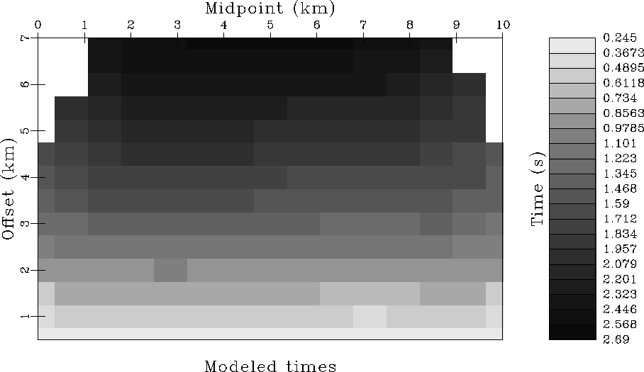
The traveltimes plotted in Figure ![[*]](http://sepwww.stanford.edu/latex2html/cross_ref_motif.gif) were integrated from the raypaths in the original model in Figure
were integrated from the raypaths in the original model in Figure ![[*]](http://sepwww.stanford.edu/latex2html/cross_ref_motif.gif) .
Traveltimes from the estimated raypaths
in Figure
.
Traveltimes from the estimated raypaths
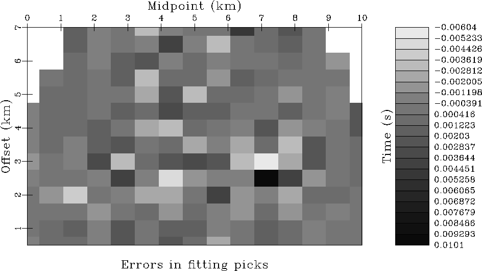
in Figure ![[*]](http://sepwww.stanford.edu/latex2html/cross_ref_motif.gif) were subtracted from
the correct traveltimes for the errors
in Figure
were subtracted from
the correct traveltimes for the errors
in Figure ![[*]](http://sepwww.stanford.edu/latex2html/cross_ref_motif.gif) . These errors ranged from
-6 ms to +10 ms, with a root-mean-square average
of 2.3 ms. Those errors which remain do not appear
to have any systematic correlation.
Such time errors are much less than would be found
at these scales in times picked from recorded surface seismic
data, where a seismic temporal wavelength
often exceeds 20 ms.
Thus, the original and estimated velocity models in
Figures
. These errors ranged from
-6 ms to +10 ms, with a root-mean-square average
of 2.3 ms. Those errors which remain do not appear
to have any systematic correlation.
Such time errors are much less than would be found
at these scales in times picked from recorded surface seismic
data, where a seismic temporal wavelength
often exceeds 20 ms.
Thus, the original and estimated velocity models in
Figures ![[*]](http://sepwww.stanford.edu/latex2html/cross_ref_motif.gif) and
and ![[*]](http://sepwww.stanford.edu/latex2html/cross_ref_motif.gif) produce effectively
indistinguishable traveltimes for this survey.
produce effectively
indistinguishable traveltimes for this survey.
 |
![[*]](http://sepwww.stanford.edu/latex2html/cross_ref_motif.gif) .
.
 |
![[*]](http://sepwww.stanford.edu/latex2html/cross_ref_motif.gif) minus
traveltimes from the estimated
model in Figures
minus
traveltimes from the estimated
model in Figures ![[*]](http://sepwww.stanford.edu/latex2html/cross_ref_motif.gif) and
and ![[*]](http://sepwww.stanford.edu/latex2html/cross_ref_motif.gif) .
The root-mean-square average of these
errors was 2.3 ms, well below any possible
accuracy in picking.
.
The root-mean-square average of these
errors was 2.3 ms, well below any possible
accuracy in picking.
Figure ![[*]](http://sepwww.stanford.edu/latex2html/cross_ref_motif.gif) shows the difference of the
original velocities in Figure
shows the difference of the
original velocities in Figure ![[*]](http://sepwww.stanford.edu/latex2html/cross_ref_motif.gif) minus the estimated velocities in Figure
minus the estimated velocities in Figure ![[*]](http://sepwww.stanford.edu/latex2html/cross_ref_motif.gif) .
The magnitudes of both anomalies has been underestimated.
Moreover, sidelobes appear about the anomalies.
The center of the estimated slow anomaly is too fast
and the edges of the slow anomaly are too slow.
The center of the estimated fast anomaly is too slow
and the edges of the fast anomaly are too fast.
Both anomalies have lost resolution in the reconstruction.
The deeper portion of the fast anomaly was missed altogether
because the original rays did not reach this depth.
.
The magnitudes of both anomalies has been underestimated.
Moreover, sidelobes appear about the anomalies.
The center of the estimated slow anomaly is too fast
and the edges of the slow anomaly are too slow.
The center of the estimated fast anomaly is too slow
and the edges of the fast anomaly are too fast.
Both anomalies have lost resolution in the reconstruction.
The deeper portion of the fast anomaly was missed altogether
because the original rays did not reach this depth.
 |
![[*]](http://sepwww.stanford.edu/latex2html/cross_ref_motif.gif) minus
the estimated velocities in figure
minus
the estimated velocities in figure ![[*]](http://sepwww.stanford.edu/latex2html/cross_ref_motif.gif) .
.
The most important application of diving wave tomography
is the correction of structural distortions in underlying
reflections. To see the effect of errors in the velocity
model, I calculate the vertical two-way traveltime from
the surface to a horizontal reflector at 2 km depth,
for all surface positions. The true velocity model
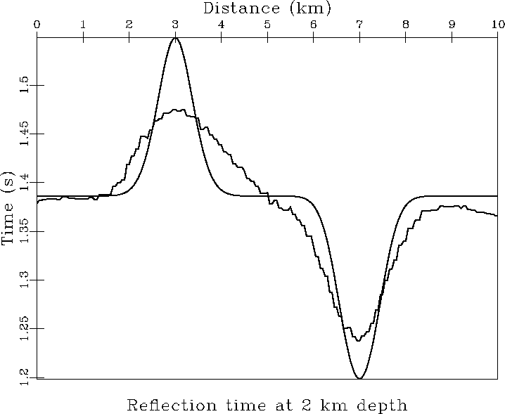
gives two distinct peaks in traveltime in Figure ![[*]](http://sepwww.stanford.edu/latex2html/cross_ref_motif.gif) ,
but the estimated velocity model gives much smoother
peaks. The positioning of peaks is correct, but lost
resolution has the effect of reducing the magnitude
of the relative changes in vertical time.
,
but the estimated velocity model gives much smoother
peaks. The positioning of peaks is correct, but lost
resolution has the effect of reducing the magnitude
of the relative changes in vertical time.
Smearing of the velocity anomalies clearly occurs parallel to the raypaths. Resolution is greatest perpendicular to the raypaths. The angular coverage of a particular anomaly is limited. Broader velocities anomalies are easier to invert than this example, but we must acknowledge this loss of resolution will affect the accuracy of our near-surface velocities. Other information, such as known shallow faults, might allow us to identify and introduce sharper edges on lateral velocity changes.
 |
![[*]](http://sepwww.stanford.edu/latex2html/cross_ref_motif.gif) .
The estimated curve has broader and shallower peaks
(time sags) than the actual curve.
.
The estimated curve has broader and shallower peaks
(time sags) than the actual curve.