A simple example of an adjoint with rough output is normal moveout.
Performing normal moveout on a trace means looping over values of vertical
travel time ![]() and solving for the appropriate travel time t.
The trace, collected at some offset, is stretched upward to simulate a zero
offset trace. Each output bin collects one
value from the input space. Performing the adjoint means pushing each
input value into an output bin. Multiple inputs
will end up in some output bins. The roughness with which the output space
samples the input space is dictated by the velocity.
and solving for the appropriate travel time t.
The trace, collected at some offset, is stretched upward to simulate a zero
offset trace. Each output bin collects one
value from the input space. Performing the adjoint means pushing each
input value into an output bin. Multiple inputs
will end up in some output bins. The roughness with which the output space
samples the input space is dictated by the velocity.
Here is a simple inversion, following an example from TDF Claerbout (1994). Begin with a single seismic trace, which we label the model, m. We also have a solution trace, labeled x, which we wish to construct from a synthetic gather d = Mm, where M is a normal moveout 0 operator, and M' its adjoint stacking operator. Thus our regression is:
| (10) |
| (11) |
We have some freedom in the way we define M and M'. M is our 0
operator, but we can choose it to sample the input trace or to sample the
output gather, and the same is true of the stacking operator M'. In order
to be precisely adjoint to each other, both M and M' must sample the
same space. Further, the mathematics of normal moveout recommend always
sampling the trace, because of the explicit relationship between vertical
travel-time ![]() and velocity. So initially we choose our NMO operator to model
by pushing values from an input trace into the output gather, and to stack
by pulling values into the trace. This gives an exact adjoint.
and velocity. So initially we choose our NMO operator to model
by pushing values from an input trace into the output gather, and to stack
by pulling values into the trace. This gives an exact adjoint.
I use this operator pair to solve the above regression and get results
as seen in Figure ![[*]](http://sepwww.stanford.edu/latex2html/cross_ref_motif.gif) . We see that the original waveforms
are reconstructed almost exactly
after just four or five iterations.
. We see that the original waveforms
are reconstructed almost exactly
after just four or five iterations.
|
results
Figure 1 Iterations of the inversion | 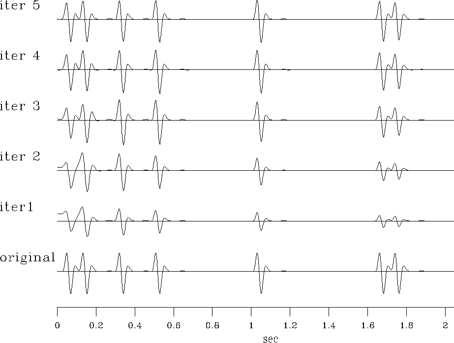 |
Now we redefine the operator. M' stays unchanged, but M is replaced. Maintaining similar naming conventions, we can define a stacking operator S which samples an input gather and pushes values into a stacked trace output. S' then must model by pulling values into the gather. We replace M by S' and obtain the regression:
| (12) |
| (13) |
Using this new operator pair in the inversion yields the results seen in
Figure ![[*]](http://sepwww.stanford.edu/latex2html/cross_ref_motif.gif) .
Amplitudes for most events are reconstructed more quickly, after a single
iteration.
.
Amplitudes for most events are reconstructed more quickly, after a single
iteration.
|
appnmo
Figure 2 Iterations of the inversion | 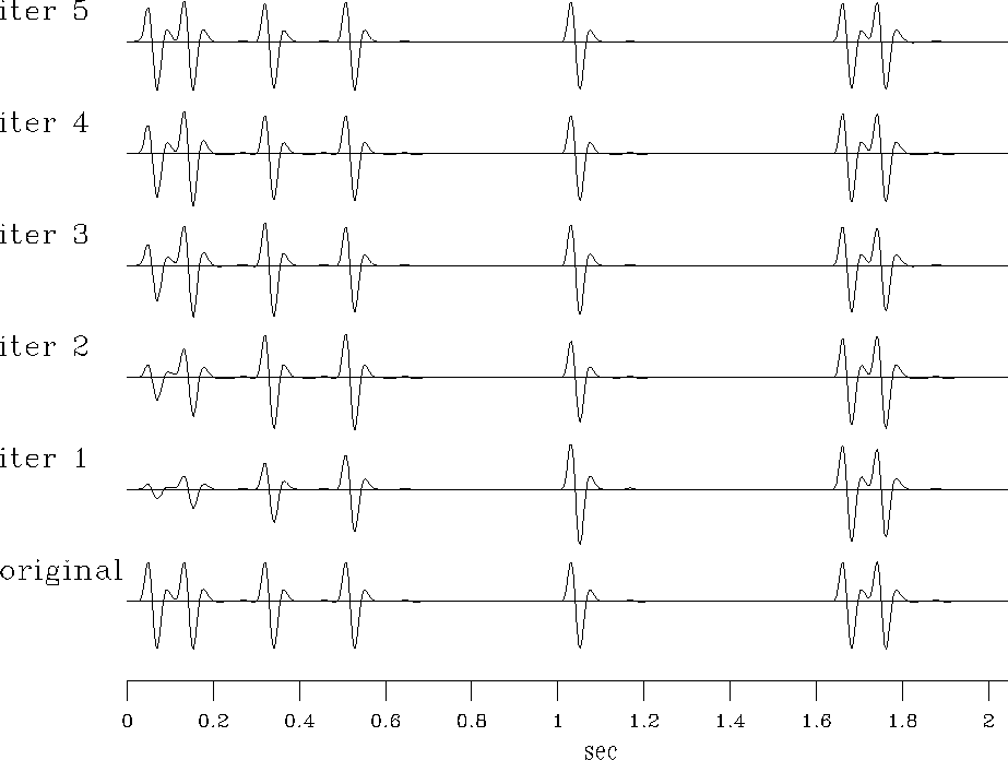 |
To quantify the results, Figure ![[*]](http://sepwww.stanford.edu/latex2html/cross_ref_motif.gif) displays the misfit of the
model at each iteration with the original trace:
displays the misfit of the
model at each iteration with the original trace: ![]() .This misfit is the model residual, normally an unknown quantity, but a useful
measure of success in synthetic problems where the exact answer is known.
The inversion which uses exclusively pull operators converges more
quickly than that which uses exact adjoints.
For this simple example, instant convergence in the model residual would mean unitarity;
accelerated convergence suggests that the pull adjoint gives something
closer to a unitary operator than the exact adjoint.
.This misfit is the model residual, normally an unknown quantity, but a useful
measure of success in synthetic problems where the exact answer is known.
The inversion which uses exclusively pull operators converges more
quickly than that which uses exact adjoints.
For this simple example, instant convergence in the model residual would mean unitarity;
accelerated convergence suggests that the pull adjoint gives something
closer to a unitary operator than the exact adjoint.
|
nmores
Figure 3 Residuals for the two inversions as a function of iteration. Dashed line denotes inversion with the exact adjoint, continuous line with the pull adjoint. | 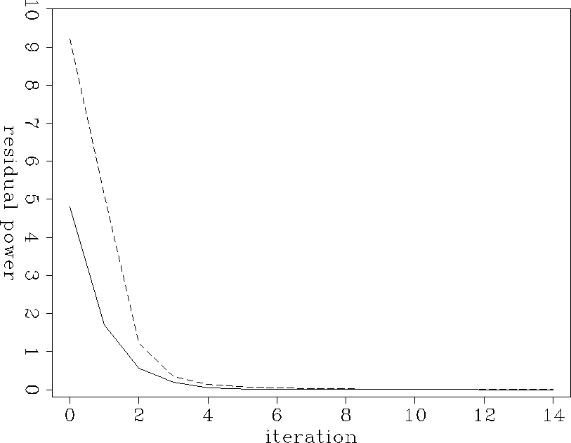 |
To satisfy curiosity, I measured data residuals (that quantity minimized
by the inversion) after several iterations at
various
slownesses. The results are shown in Figure ![[*]](http://sepwww.stanford.edu/latex2html/cross_ref_motif.gif) . The smooth
curve corresponds to the pull adjoint and the rough one to the exact
adjoint.
At all velocities, there is a noticeable advantage to using pull adjoint
NMO.
It is surprising that there is so little velocity dependence,
because it seems the aliasing at high dips (or low velocities)
should be a problem for push operators more than for pull operators.
Further, the magnitude by which the operator pair which includes
the pull adjoint fails the dot product test is not systematically
dependent on velocity.
. The smooth
curve corresponds to the pull adjoint and the rough one to the exact
adjoint.
At all velocities, there is a noticeable advantage to using pull adjoint
NMO.
It is surprising that there is so little velocity dependence,
because it seems the aliasing at high dips (or low velocities)
should be a problem for push operators more than for pull operators.
Further, the magnitude by which the operator pair which includes
the pull adjoint fails the dot product test is not systematically
dependent on velocity.
|
slowres
Figure 4 Comparison of residual after one iteration for the pull and exact adjoint. The smooth curve denotes the pull adjoint. Click to see movie of residuals at higher numbers of iterations. | 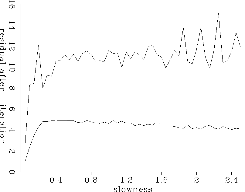 |
|
dotprods
Figure 5 Error in the dot product test is independent of velocity. | 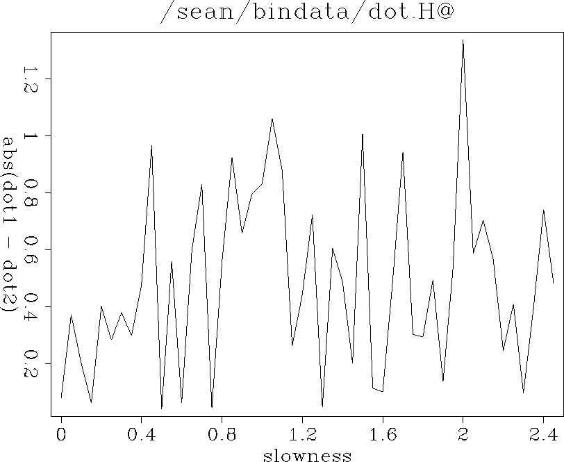 |