Migration results

The superposition of the migrated results onto the velocity model (Figure ) shows that common-azimuth migration successfully imaged the reflectors and correctly positioned them in depth. The migrated salt boundaries overlap quite precisely with the salt boundaries identified by the sharp variations in the velocity model. The target reflectors below the salt layer are also well imaged, though it seems that their focusing could be improved by further refinements of the velocity function. When the same velocity function used for common-azimuth migration was used for 3-D prestack Kirchhoff depth migration small residual moveout corrections of the migrated CRP gathers were required to maximize the image energy.

The accuracy of common-azimuth migration can be analyzed in more detail by plotting smaller sections of the data, and compare the results of full 3-D prestack migration with multi-line 2-D prestack migration. The difference between the two results are mostly visible in the cross-line sections, where the lack of focusing in the multi-line 2-D migration results manifests itself. In the following sequence of figures I show three cross-line sections located at the left-edge, in the middle, and at the right edge, of the central fault system. Figure  shows the comparison of the common-azimuth migration (left) and of the multi-line 2-D migration (right) for the same cross-line. 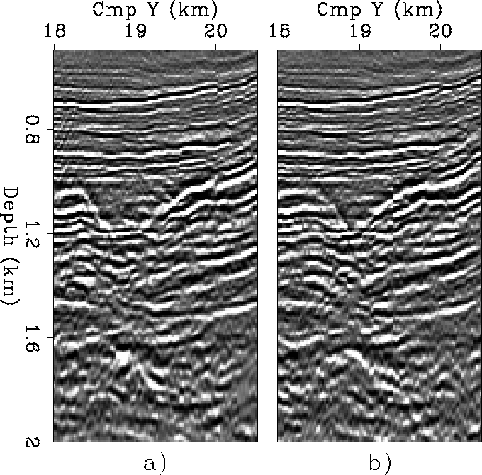The most obvious differences between the two sections are in the reflections from the boundary between the Jurassic and the Triassic formations, located at about 1.1 km in depth. Common-azimuth correctly positioned the lithological boundary, while multi-line 2-D migration mispositioned the boundaries by several hundred meters and did not properly focus the reflector. The lack of focusing in the cross-line direction prevents multi-line 2-D migration from properly imaging the top of the salt layer, visible in Figure  at a depth of about 1.6 km. Unfocused diffractions are clearly visible in the multi-line 2-D migration results (right panel in the figure). On the other hand, common-azimuth migration (left) nicely images the roughness at the top of the salt. 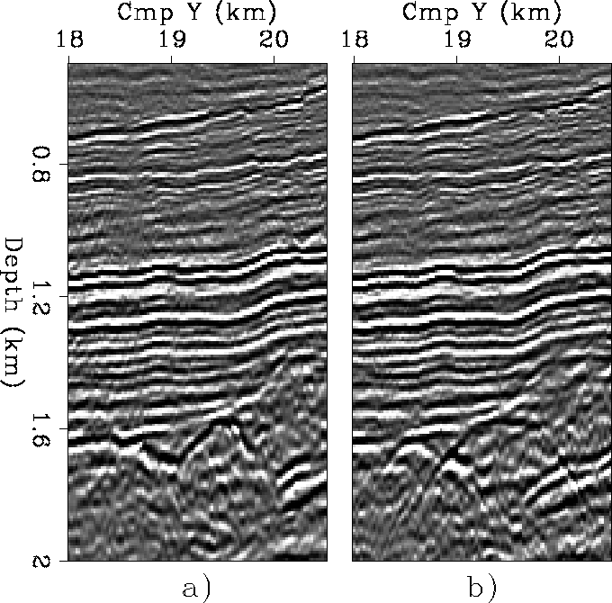A similar situation is shown in the cross-line sections of Figure . Common-azimuth migration correctly focuses the diffractions caused by the uneven top of the salt, as well as the diffractions caused by the shallow faults visible at the top-right corner of the sections.

 

x16088
Figure 3 Migrated cross-line sections (CMP X=16.088 km) obtained by a) 3-D common-azimuth migration, b) multi-line 2-D migration.

 

x16566
Figure 4 Migrated cross-line sections (CMP X=16.566 km) obtained by a) 3-D common-azimuth migration, b) multi-line 2-D migration.

 

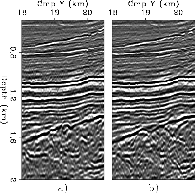
x16820
Figure 5 Migrated cross-line sections (CMP X=16.82 km) obtained by a) 3-D common-azimuth migration, b) multi-line 2-D migration.

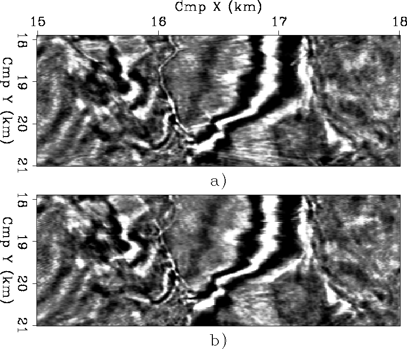
The lack of cross-line focusing in the multi-line 2-D migration is also evident in the depth slices shown in Figure . These depth slices, taken at a depth of 1.096 km, clearly show the reflections from the boundary between the Jurassic and the Triassic formations around the in-line midpoint location of 16 km. This is the same event previously shown in the cross-line sections of Figure . Examining this depth slice we can verify that common-azimuth migration correctly positions the reflection at the true boundary between the formations, while multi-line 2-D migrations mispositions the boundary, even transforming it in a bowtie-shaped event around the cross-line midpoint location of 19 km. The set of faults cutting across the broad reflection located between 16.5 km and 17 km in the in-line direction is also more sharply imaged by common-azimuth migration than by multi-line 2-D migration.

 

z1096
Figure 6 Migrated depth slices (Z=1.096 km) obtained by a) 3-D common-azimuth migration, b) multi-line 2-D migration.

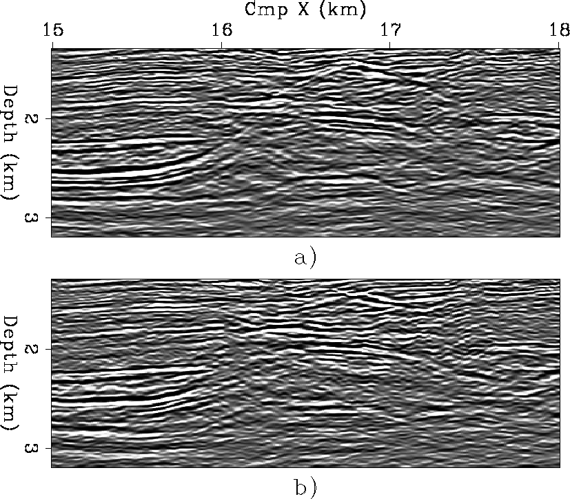
Figure  compares the results of common-azimuth migration (top) and multi-line 2-D migration (bottom) when imaging the salt layer and the target reflectors below it. The salt boundaries are fairly well imaged by common-azimuth migration, including the bottom of the salt and part of the salt flanks. I expect that a dip-preserving transformation to common-azimuth that includes AMO in the processing sequence would improve the imaging of the steeply dipping salt flanks. The reflectors below the reservoir are well imaged, although with uneven amplitudes. Refinements in the velocity model may improve the imaging of these reflectors. On the contrary, the multi-line 2-D migration poorly images the bottom of the salt layer and the reflector below the salt. The salt flanks are almost totally lost in the multi-line 2-D migration image as well. Two effects play a role to cause the large differences between the two migrations when imaging reflectors that have a fairly mild cross-line dip component. First, the large width of the cross-line migration aperture at this depth makes the images very sensitive to cross-line dips. Second, common-azimuth migration correctly takes into account the cross-line velocity variations because it correctly propagates the wavefield in the cross-line direction as well in the in-line direction. On the contrary, multi-line 2-D migration constrains the wavefield to propagate along the vertical in-line planes, and cannot fully honor the 3-D nature of the velocity function.

 

y20000
Figure 7 In-line sections (CMP Y=20 km) obtained by a) 3-D common-azimuth migration, b) multi-line 2-D migration.