Next: Frequency Domain Formulation
Up: BEAM STACK
Previous: BEAM STACK
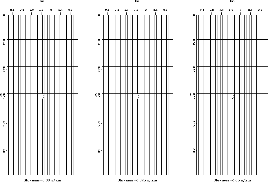
Each of the three panels in figure ![[*]](http://sepwww.stanford.edu/latex2html/cross_ref_motif.gif) represents a slice of an example beam stack model space with constant slowness.
Together these three slices constitute an entire beam stack model space
with slowness parameters: p1=0.0s/km,p2=0.025s/km,p3=0.5s/km. The energy in
this model space is zero at all locations except three
points. The forward operation applied to the model space
will map the nonzero energy in model space to the parabolic
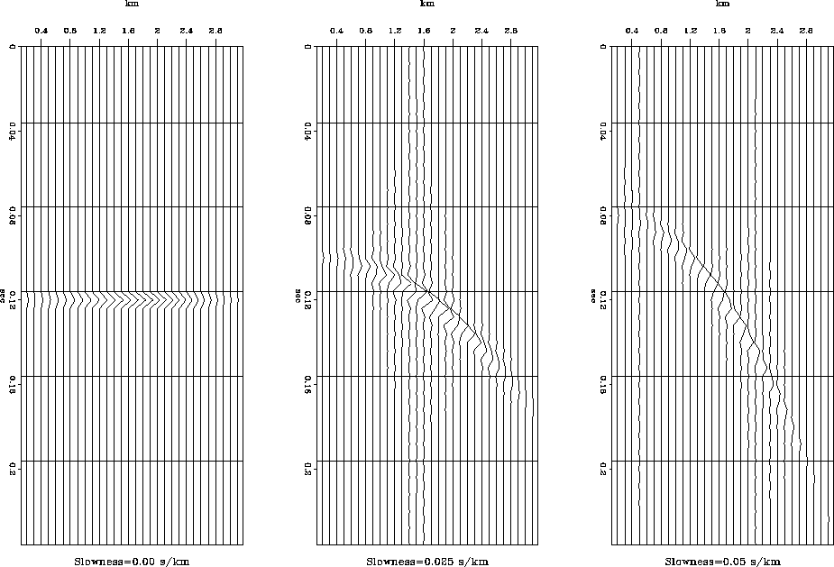
trajectories in data space illustrated in figure .
The left panel of figure corresponds to the zero
slowness slice, p=0s/km, and as such the point with nonzero energy maps to the zero
dip trajectory that is displayed on the left of figure .
The middle panel
corresponds to the slowness slice p=0.025s/km and maps the point of nonzero
energy to the trajectory displayed in the middle row of figure .
The right panel of figure corresponds the
slowness slice p=0.05s/km and
maps the point of nonzero energy to the trajectory at the right in figure
. Figure illustrates the
forward mapping from individual points in model space. These three
trajectories in themselves do not constitute the complete mapping to
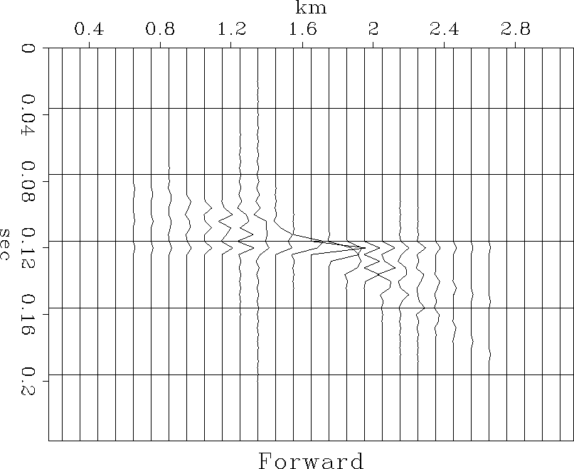
model space; to
obtain the complete forward modeling, each forward mapping
from individual points in model space must be summed together. This
is displayed in figure . This data has multi-valued dips
at the t-x location (0.12,1.6).
Unraveling multi-valued dips is one of the problems that
needs to be addressed in modeling multiples and primaries.
represents a slice of an example beam stack model space with constant slowness.
Together these three slices constitute an entire beam stack model space
with slowness parameters: p1=0.0s/km,p2=0.025s/km,p3=0.5s/km. The energy in
this model space is zero at all locations except three
points. The forward operation applied to the model space
will map the nonzero energy in model space to the parabolic
trajectories in data space illustrated in figure .
The left panel of figure corresponds to the zero
slowness slice, p=0s/km, and as such the point with nonzero energy maps to the zero
dip trajectory that is displayed on the left of figure .
The middle panel
corresponds to the slowness slice p=0.025s/km and maps the point of nonzero
energy to the trajectory displayed in the middle row of figure .
The right panel of figure corresponds the
slowness slice p=0.05s/km and
maps the point of nonzero energy to the trajectory at the right in figure
. Figure illustrates the
forward mapping from individual points in model space. These three
trajectories in themselves do not constitute the complete mapping to
model space; to
obtain the complete forward modeling, each forward mapping
from individual points in model space must be summed together. This
is displayed in figure . This data has multi-valued dips
at the t-x location (0.12,1.6).
Unraveling multi-valued dips is one of the problems that
needs to be addressed in modeling multiples and primaries.
The adjoint operation maps the data that lies on the trajectories
displayed in figure back to the model space. The
complete adjoint operation sums over trajectories for each location in
data space. The beam stack operator is not unitary and as such, the mapping of
the result of the forward operation, mentioned above and displayed in
figure , will not map exactly back to the original
model displayed in figure . The result of the adjoint operation applied to
the data displayed in figure is displayed in figure .
The great disparity between the original model displayed in
figure and the adjoint applied to the forward modeled data
displayed in figure is a consequence of the original model chosen.
The original model includes points of energy, which are not a natural
representation of events in beam stack model space. The beam stack
transform models dips which necessarily have a greater extent than a
point. I chose this model to illustrate what a beam stack trajectory
looks like and to illustrate the relation between the model and data space.
model
Figure 1 Example model space of the beam stack
transform. Slowness values are p1=0.0s/km,p2=0.025s/km,p3=0.05s/km.


 stakTraj
Figure 2 Trajectories resulting from the
forward modeling of each of the non-zero points individually in the
example model space.
data
Figure 3 Data resulting from the forward
modeling of the example model space.
adj
Figure 4 Adjoint operation applied to the
forward modeled example model space.
Next: Frequency Domain Formulation
Up: BEAM STACK
Previous: BEAM STACK
Stanford Exploration Project
11/11/1997