APPLICATION

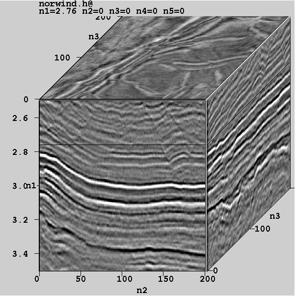
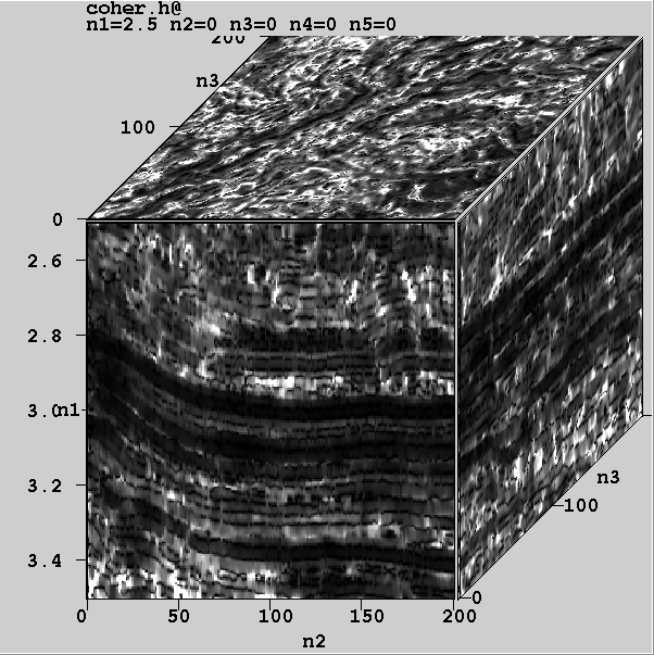
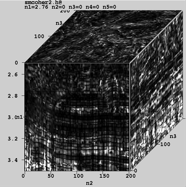
Figure 1 is a 3-D view of a small data volume with good local plane wave behavior. While faults with large throw are clearly visible, those with smaller displacement are not. Equation (5) with a three point spatial and a 44 millisecond temporal smoother, was used to derive the dip-magnitude cube shown in Figure 2. Figure 2 is indicative of the fact that typical cross-sectional views of dip-magnitude cubes are not pleasing and reveal little about potential interesting events in the data.

 

Fig1
Figure 1 Original 3-D Data Volume

 

Fig2
Figure 2 Dip Magnitude 3-D Data Volume

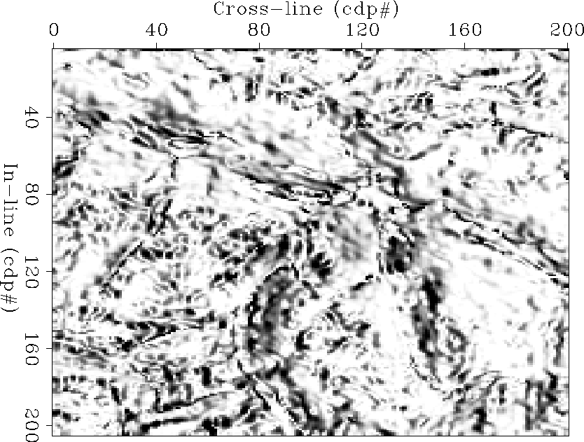
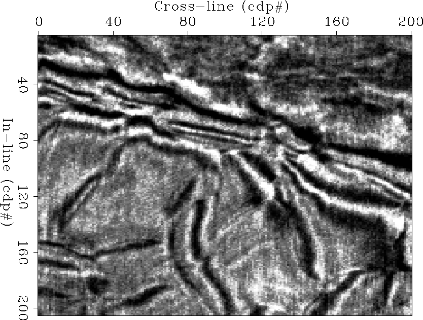
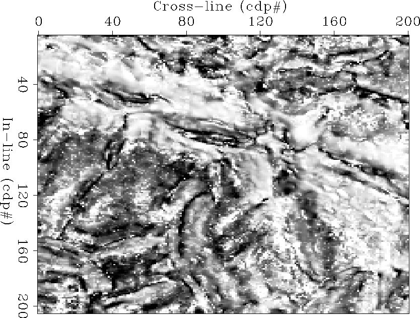
Figure 3 is a time slice through the dip-magnitude data set at 2.76 seconds. It should be compared with the equivalent input time slice in Figure 4. Interesting anamolies are now easily recognized. A careful review of the dip-magnitude volume shows that many low resolution events are highlighted and much more easily recognized. The availability of dip-magnitude data has certainly increased the overall information content.

 

fig3
Figure 3 Dip Magnitude Slice at 2.76 Seconds

 

fig4
Figure 4 Original Slice at 2.76 Seconds

 

fig5
Figure 5 Coherency Slice at 2.76 Seconds

 

Fig6
Figure 6 Coherency 3-D data Volume