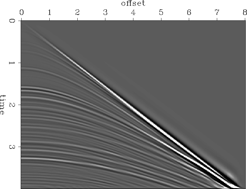
We constructed a synthetic interval velocity model, and then modeled
a CMP gather using a finite difference code, Figure ![[*]](http://sepwww.stanford.edu/latex2html/cross_ref_motif.gif) .
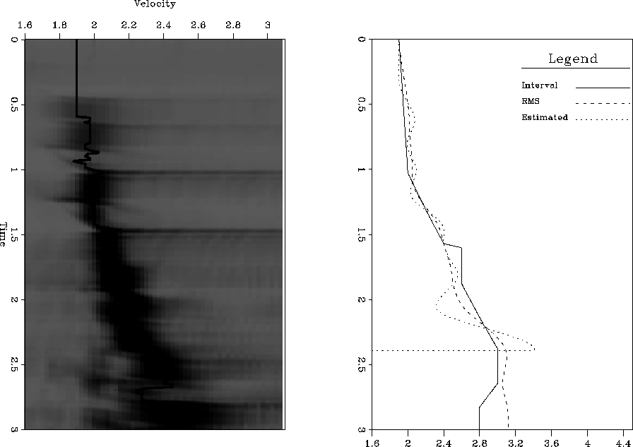
We then picked RMS velocities and attempted to estimate our interval velocity.
As Figure
.
We then picked RMS velocities and attempted to estimate our interval velocity.
As Figure ![[*]](http://sepwww.stanford.edu/latex2html/cross_ref_motif.gif) shows, we did a very good job of recovering
the correct interval velocity.
shows, we did a very good job of recovering
the correct interval velocity.
|
synthetic-data
Figure 6 Modeled synthetic data. |  |
|
synthetic
Figure 7 Initial interval velocity, picked RMS curve, and inverted interval velocity curve. |  |
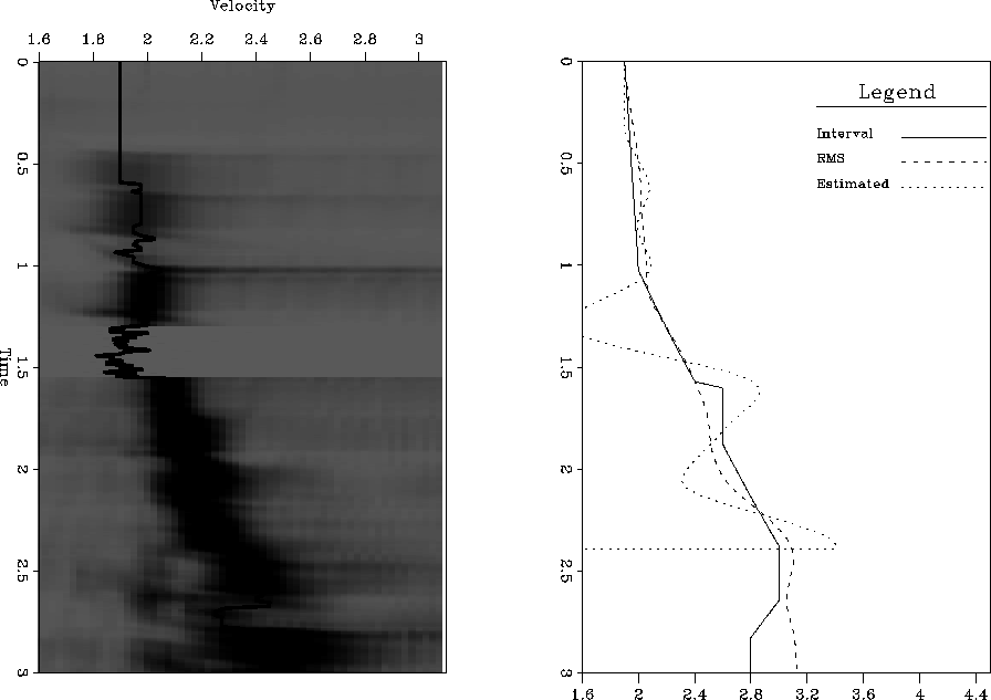
Using the same dataset (Figure ![[*]](http://sepwww.stanford.edu/latex2html/cross_ref_motif.gif) ) we introduced some
low-energy noise to our velocity scan and then attempted to invert back
to our interval velocities. As Figure
) we introduced some
low-energy noise to our velocity scan and then attempted to invert back
to our interval velocities. As Figure ![[*]](http://sepwww.stanford.edu/latex2html/cross_ref_motif.gif) shows, even with the grossly
inaccurate RMS picks at approximately 1.5 seconds we were still able
to recover a reasonable interval velocity curve.
shows, even with the grossly
inaccurate RMS picks at approximately 1.5 seconds we were still able
to recover a reasonable interval velocity curve.
|
gap
Figure 8 Left panel, RMS picks overlaying semblance scan with noise introduced at approximately 1.5 seconds. Right panel, the resulting interval velocity curve, the curve without the bad data, and our bad-data RMS curve. |  |
|
xvals
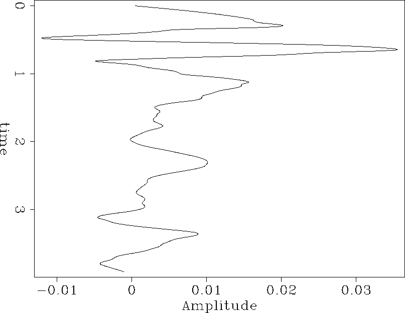
Figure 9 Our preconditioned variable for the continuous case. |  |