


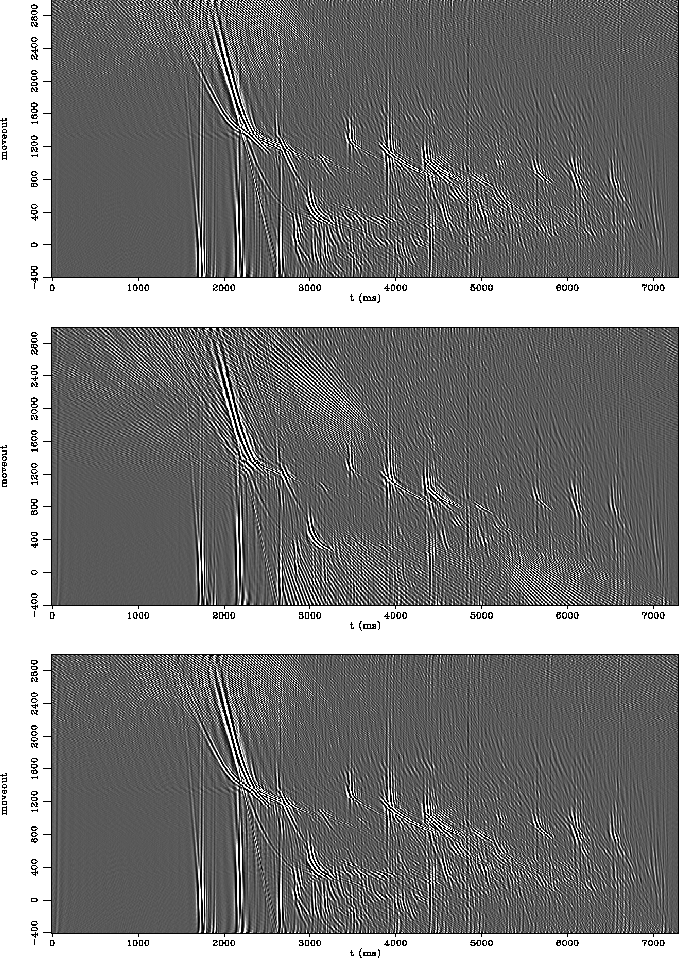
Results sorted into an example CMP gather and windowed are shown in Figures compWin0. The left side shows the original data, the center shows the output after throwing out every other offset and interpolating with local volume prediction error filters, and the right side shows the residual clipped for comparison. Figure compWin0 is a window from the near offset traces. Here the data have noticeable curvature, and so they are difficult to predict and there is some energy in the residual. Happily, energetic events are reconstructed with good fidelity. At farther offsets (not shown), where events tend to become much more linear, the residual vanishes completely.
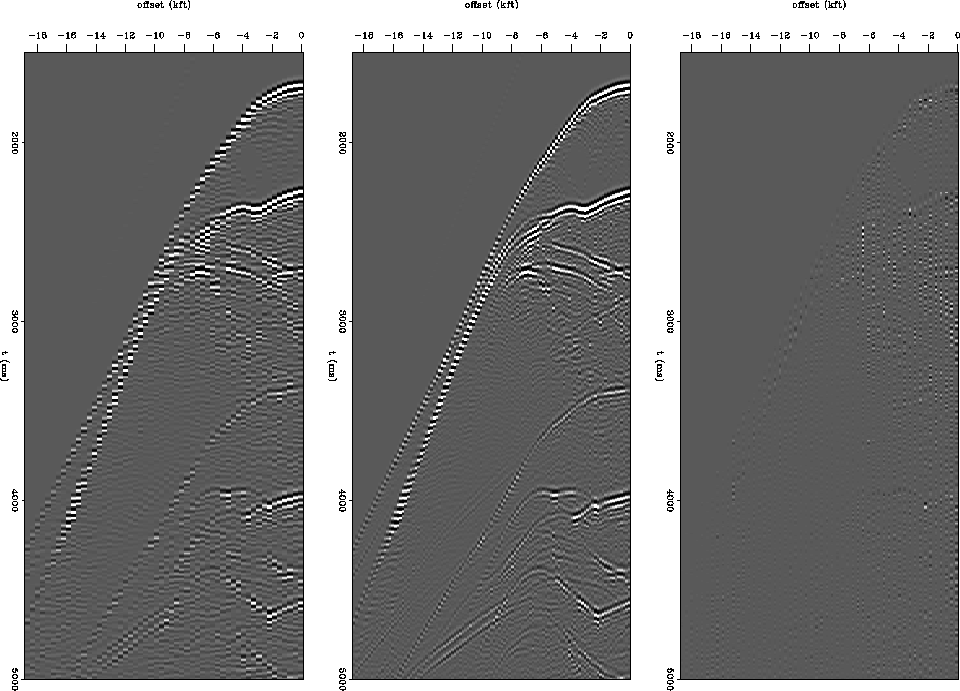 |


Because the motivation for resampling in this case is multiple suppression, Figure cr90 shows portions of parabolic radon transforms for these same data. In these figures the left shows the radon transform of the original data, the center shows the transform of the decimated data, and the right shows the transform of the reinterpolated data. The center panel shows that the primaries in the decimated data are poorly represented in the radon transform, especially in the complex area around 2.5 to 3.7 seconds. The decimated data also shows more artifact energy in the multiple region of the transform. The original and interpolated data produce better radon transforms.
CMP gathers after radon demultiple are shown in Figure compCmp. The left panel shows a portion of a CMP gather with alternate offsets removed and radon demultiple applied. The right panel shows the same portion with the removed offsets reinterpolated, radon demultiple applied, and the interpolated traces thrown away. The left panel shows less suppression of various multiple events, most notably the steep multiples labeled A, and also some attenuation of primary energy, such as at B.
Figure compStack shows a subsalt portion of a stacked section. The left panel shows the result of radon demultiple and stack on the decimated data, the right panel shows the result of simple stack on the interpolated data. The reason for the difference in flow is that simply stacking the data which has been dealiased by interpolation (leaving out the innermost few traces) removes most of the multiple energy, but doing a similar operation on the decimated data (left panel) gives a terrible result, because the aliased nature of the multiples causes them to come through in the stack as a short-period (50ms or so) series of seafloor multiples that completely obscures the section. At any rate, the right panel is approximately identical with or without going to the trouble of radon transform. Strong multiple events (examples at A) are suppressed more or less equivalently in the two sections; arguably somewhat better in the interpolated data. Some important primaries at B are significantly attenuated in the decimated data, as shown by comparison with the interpolated data. Also, throughout the section, most visible in the neighborhood of C, aliasing results in layer-like artifacts. Finally, many interesting arrivals, especially diffractions, in the faulted area around D are strongly attenuated in the decimated data.
 |