

Next: Three codes for inverse
Up: EMPTY BINS AND PRECONDITIONING
Previous: EMPTY BINS AND PRECONDITIONING
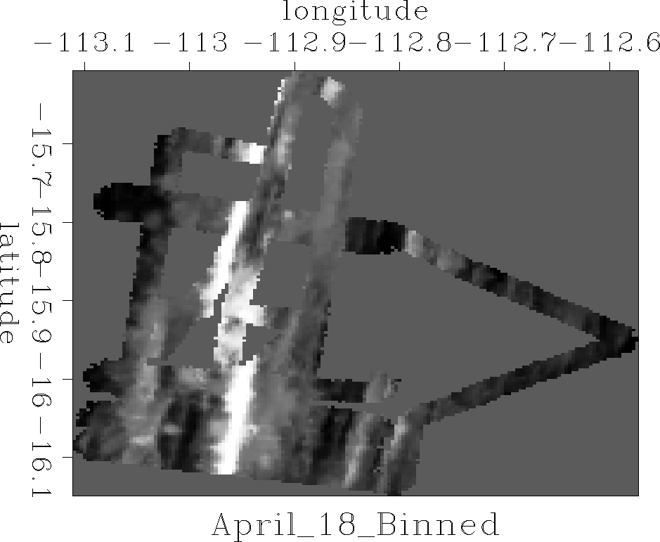
Figure ![[*]](http://sepwww.stanford.edu/latex2html/cross_ref_motif.gif) shows a day's worth of data
shows a day's worth of data![[*]](http://sepwww.stanford.edu/latex2html/foot_motif.gif) collected at sea by SeaBeam,
an apparatus for measuring water depth both
directly under a ship, and somewhat off to the sides of the ship's track.
The data is measurements of depth h(x,y) at miscellaneous locations
in the (x,y)-plane.
collected at sea by SeaBeam,
an apparatus for measuring water depth both
directly under a ship, and somewhat off to the sides of the ship's track.
The data is measurements of depth h(x,y) at miscellaneous locations
in the (x,y)-plane.
seabin90
Figure 8
Depth of the ocean under ship tracks.
Empty bins are displayed with an average depth  . . |
|  |


The locations are scattered about,
according to various aspects
of the ship's navigation and the geometry of the SeaBeam sonic antenna.
Figure ![[*]](http://sepwww.stanford.edu/latex2html/cross_ref_motif.gif) was made by binning with
bin2()
was made by binning with
bin2() ![[*]](http://sepwww.stanford.edu/latex2html/cross_ref_motif.gif) and equation (
and equation (![[*]](http://sepwww.stanford.edu/latex2html/cross_ref_motif.gif) ).
The spatial spectra of the noise in the data
could be estimated where tracks cross over themselves.
This might be worth while, but we do not pursue it now.
).
The spatial spectra of the noise in the data
could be estimated where tracks cross over themselves.
This might be worth while, but we do not pursue it now.
Here we focus on the empty mesh locations where no data is recorded
(displayed with the value of the mean depth  ).
These empty bins were filled with
module mis2
 ![[*]](http://sepwww.stanford.edu/latex2html/cross_ref_motif.gif) .
Results are in Figure
.
Results are in Figure ![[*]](http://sepwww.stanford.edu/latex2html/cross_ref_motif.gif) .
.
prcfill
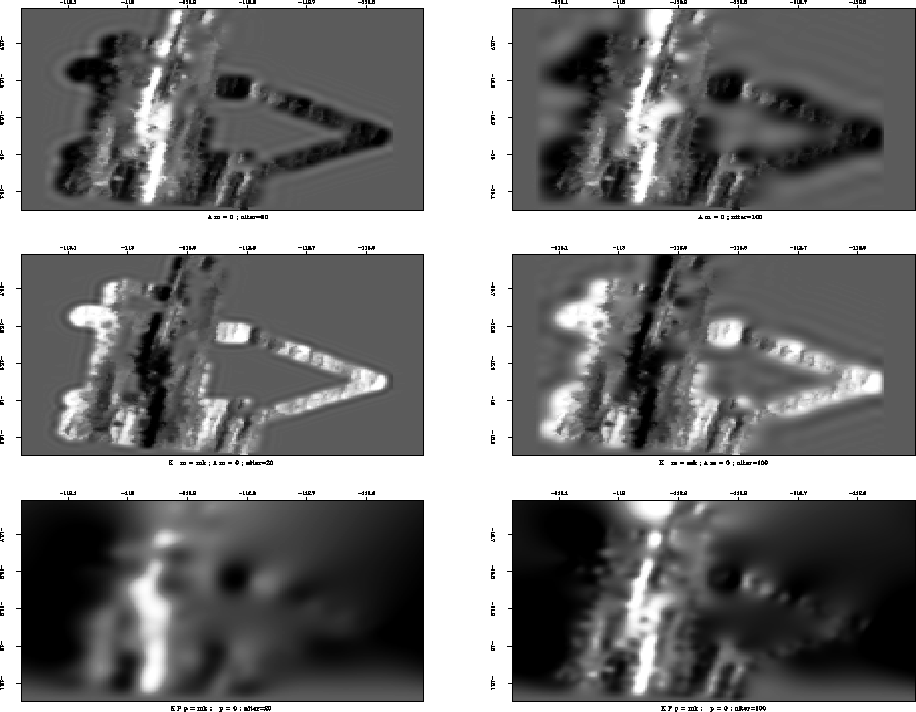
Figure 9
The ocean bottom restoring missing data with a helix derivative.
![[*]](http://sepwww.stanford.edu/latex2html/movie.gif)


In Figure ![[*]](http://sepwww.stanford.edu/latex2html/cross_ref_motif.gif) the left column results from 20 iterations
while the right column results from 100 iterations.
the left column results from 20 iterations
while the right column results from 100 iterations.
The top row in Figure ![[*]](http://sepwww.stanford.edu/latex2html/cross_ref_motif.gif) shows that more iterations
spreads information further into the region of missing data.
shows that more iterations
spreads information further into the region of missing data.
It turned out that the original method strictly honoring known data
gave results so similar to the second method (regularizing)
that the plots could not be visually distinguished.
The middle row in Figure ![[*]](http://sepwww.stanford.edu/latex2html/cross_ref_motif.gif) therefore shows
the difference in the result of the two methods.
We see an outline of the transition between known and unknown regions.
Obviously, the missing data is pulling known data towards zero.
therefore shows
the difference in the result of the two methods.
We see an outline of the transition between known and unknown regions.
Obviously, the missing data is pulling known data towards zero.
The bottom row in Figure ![[*]](http://sepwww.stanford.edu/latex2html/cross_ref_motif.gif) shows that preconditioning
spreads information to great distances much quicker
but early iterations make little effort to honor the data.
(Even though these results are for
shows that preconditioning
spreads information to great distances much quicker
but early iterations make little effort to honor the data.
(Even though these results are for  .)
Later iterations make little change at long distance
but begin to restore sharp details on the small features
of the known topography.
What if we can only afford 100 iterations?
Perhaps we should first do 50 iterations with
preconditioning to develop the remote part of the solution and
then do 50 iterations by one of the other two methods to be sure
we attended to the details near the known data.
A more unified approach (not yet tried, as far as I know)
would be to unify the techniques.
The conjugate direction method searches two directions,
the gradient and the previous step.
We could add a third direction,
the smart direction of equation (14).
Instead of having a  matrix
solution like equation (
matrix
solution like equation (![[*]](http://sepwww.stanford.edu/latex2html/cross_ref_motif.gif) ) for two distances,
we would need to solve a
) for two distances,
we would need to solve a  matrix for three.
Figure ![[*]](http://sepwww.stanford.edu/latex2html/cross_ref_motif.gif) has a few artifacts connected with the
use of the helix derivative.
Examine equation (
has a few artifacts connected with the
use of the helix derivative.
Examine equation (![[*]](http://sepwww.stanford.edu/latex2html/cross_ref_motif.gif) ) to notice the shape of the helix derivative.
In principle, it is infinitely long in the horizontal axis
in both equation (
) to notice the shape of the helix derivative.
In principle, it is infinitely long in the horizontal axis
in both equation (![[*]](http://sepwww.stanford.edu/latex2html/cross_ref_motif.gif) ) and Figure
) and Figure ![[*]](http://sepwww.stanford.edu/latex2html/cross_ref_motif.gif) .
In practice, it is truncated. The truncation is visible as bands
along the sides of Figure
.
In practice, it is truncated. The truncation is visible as bands
along the sides of Figure ![[*]](http://sepwww.stanford.edu/latex2html/cross_ref_motif.gif) .
.
As a practical matter, no one would use the first two bin filling methods
with helix derivative for the roughener
because it is theoretically equivalent to the gradient operator
 which has many fewer coefficients.
Later, in Chapter
![[*]](http://sepwww.stanford.edu/latex2html/cross_ref_motif.gif) we'll find a much smarter roughening operator
we'll find a much smarter roughening operator  called the Prediction Error Filter (PEF)
which gives better results.


Next: Three codes for inverse
Up: EMPTY BINS AND PRECONDITIONING
Previous: EMPTY BINS AND PRECONDITIONING
Stanford Exploration Project
4/27/2004
![[*]](http://sepwww.stanford.edu/latex2html/cross_ref_motif.gif) shows a day's worth of data
shows a day's worth of data![[*]](http://sepwww.stanford.edu/latex2html/foot_motif.gif) collected at sea by SeaBeam,
an apparatus for measuring water depth both
directly under a ship, and somewhat off to the sides of the ship's track.
The data is measurements of depth h(x,y) at miscellaneous locations
in the (x,y)-plane.
collected at sea by SeaBeam,
an apparatus for measuring water depth both
directly under a ship, and somewhat off to the sides of the ship's track.
The data is measurements of depth h(x,y) at miscellaneous locations
in the (x,y)-plane.


![[*]](http://sepwww.stanford.edu/latex2html/movie.gif)